 |
|
|
|
|
||
A Field Theory Demonstrating |
Purpose
The purpose of the Nuclear Gravitation Field Theory is to demonstrate that the Strong Nuclear Force and gravity are one and the same using Quantum Mechanics, Newton’s Law of Gravity, and Einstein’s General Relativity Theory.
Ground Rules
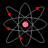
If the Strong Nuclear Force is Gravity, then the Nuclear Gravitation Field must initially be a stronger field of attraction than the Coulombic repulsive field of the Nuclear Electric Field tending to repel Protons from the Nucleus.
If the Strong Nuclear Force is Gravity, then the Nuclear Gravitation Field should propagate in all directions outward from the Nucleus of the Atom to infinity.
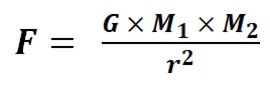
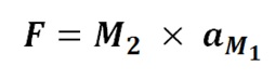
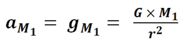
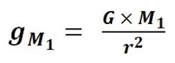
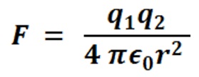
If the Strong Nuclear Force is Gravity and the Classical Physics shape of the Nucleus forms a near perfect sphere, then the Nuclear Gravitation Field should propagate outward from the Nucleus omnidirectional with spherical symmetry to infinity. In this case, the Nuclear Gravitation Field intensity should drop off as a function of 1/r2 in like manner to Newton’s Law of Gravity where r is the distance from the center of the Nucleus to the center of the Proton or Neutron being evaluated. The first equation mathematically defines Newton’s Law of Gravity where F is the gravitational force of attraction between spherical mass M1 and spherical mass M2, G is the Universal Gravitation Constant, and r is the distance between the center of mass M1 and center of mass M2. The second and third equations evaluate the acceleration field aM1 equal to the gravitational field gM1 of mass M1 acting upon mass M2.
Classical Mechanics excluding Quantum Mechanics states:
Total Energy = Kinetic Energy + Potential Energy
TE = KE + PE
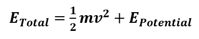
Quantum Mechanics uses the Schrodinger Wave Equation to evaluate total energy of an atomic or nuclear particle such as the electron, proton, or neutron. The general form of the equation is as follows:
Total Energy = Kinetic Energy + Potential Energy

Where the General Schrodinger Wave Equation is defined in Spherical Coordinates: i is the square root of −1, h-bar is Planck’s Constant, h, divided by 2π, ∂ is the first order partial derivative operator, ψ is the wave function of the particle being evaluated, ∇2 is the second order spatial derivative operator, r is the distance from the center of the Nucleus to the center of the particle being evaluated, θ is the azimuthal angle of the particle being evaluated relative to the Nucleus from 0 to 2π radians, φ is the altitude angle of the particle being evaluated relative to the Nucleus from –π/2 to +π/2 radians, t is time, m is the mass of the particle being evaluated, V is the general Potential Function operating on particle wave function ψ.
If the field provides an acting force on a particle where Force is proportional to 1/r2, then the Potential Energy of that particle can be determined by integrating that Force over a given distance. The Potential Energy (PE) function will be proportional to 1/r, where r is the variable in the Potential Energy Function incorporated in the Schrodinger Wave Equation:.
Force x Distance = Work or Energy The following equations represent a generic Force proportional to 1/r2, r being the distance of the particle from the center of the Force acting upon the particle and the resultant Potential Energy proportional to 1/r.
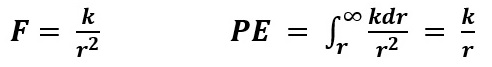
By convention, the Potential Energy for a particle “bound” within a system is considered a negative value. The particle is no longer “bound” by the system at the point where the Potential Energy is equal to zero. This occurs when the particle is at a distance of infinity or “∞” from the system. Whether we consider the Electron bound to the Nucleus of the Atom by the Nuclear Electric Field or the Proton or Neutron bound to the Nucleus by the Nuclear Gravitation Field, the Potential Energy Function will be determined by integrating the Force from a distance r from the Nucleus to the distance where the particle is no longer bound or ∞.
The following equations represent the Nuclear Electric Field Force and Potential Energy of an Electron orbiting a Nucleus with Z number of Protons where e represents the electric charge of an Electron or Proton and r represents the Electron distance from the center of the Nucleus:

The following equations represent the Nuclear Gravitation Field Force and Potential Energy of either a Proton or Neutron added to a Nucleus with Z number of Protons and N number of Neutrons where mp or n represents mass of the proton or neutron and r represents the proton or neutron distance from the center of the Nucleus:

The Schrodinger Wave Equation for the Nuclear Electric Field Potential is a Quantum Mechanical Analysis of the electron in position around a given Nucleus. This equation assumes the Nucleus is a point source of the Electric Field because the radius of the Atom containing the electrons range from 30,000 to 100,000 times the radius on the Nucleus. Therefore, the Nuclear Electric Field appears to propagate outward from the Nucleus omnidirectional with spherical symmetry to infinity. The Nuclear Electric Field intensity drops off as a function of 1/r2 where r is the distance of the Electron being evaluated from the center of the Nucleus. The Schrodinger Wave Equation for the Total Energy of the electron of interest being evaluated about the Nucleus with its Potential Energy as a function of 1/r is as follows:

Where m represents the mass of an electron, Z represents the number of Protons in the Nucleus, e represents the value of electric charge of a single Proton or single Electron, and ∈0 is the permittivity of the Electric Field in free space.
The solutions to the Schrodinger Wave Equation for the Nuclear Electric Field Potential are known, define how the electron energy levels are filled about the Nucleus, and produce the Periodic Table of the Elements which define the chemical properties of those elements. The solutions to the Schrodinger Wave Equation for the Nuclear Electric Field establish how each of the energy levels fill with Electrons if the function used to provide Electron Potential Energy is proportional to 1/r.
When the Nucleus of the Atom meets a classical physical configuration that supports a Nuclear Gravitation Field propagating outward omnidirectional with spherical symmetry where the Nuclear Gravitation Field propagates outward proportional to 1/r2, then the associated Schrodinger Wave Equation will have a Gravitational Field Potential Energy for either the Proton or Neutron being evaluated proportional to 1/r and the following form of the Schrodinger Wave Equation can be considered valid.

It is expected that all the applicable energy levels for Protons and Neutrons will fill in identical manner as the same applicable energy levels for Electrons are filled. For the Schrodinger Wave Equation for the Nuclear Gravitation Field::&nsp; G is the Universal Gravitation Constant, Z is the number of Protons in the Nucleus, mp is the mass of a Proton, N is the number of Neutrons in the Nucleus, mn is the mass of a Neutron, and mp or n represents mass of the Proton or Neutron being added to the Nucleus.
NOTE:
The constant G would be consistent with the Universal Gravitation Constant outside the Electron cloud. The value of G within the Nucleus of the Atom may very well be 1050 times larger considering that the Strong Nuclear Force and gravity are quantized. If the Strong Nuclear Force is Gravity and the calculated Nuclear Gravitation Field intensity at the surface of the Nucleus of the Atom is greater than or equal to the gravity field of our Sun, then the General Relativity effect of Space-Time Compression must be considered to take place.
If the Strong Nuclear Force is Gravity, then the Nuclear Gravitation Field must be associated with specific energy levels of the Protons and Neutrons in the Nucleus of the Atom, therefore, must be considered quantized because the Nuclear Gravitation Field intensity is concentrated at specific energy level spectral lines. The quantized Nuclear Gravitation Field intensity versus the average gravity field intensity should be analogous to a quantized photon of energy to the average energy from light distributed evenly upon a surface.
If the Strong Nuclear Force is Gravity, the Nuclear Gravitation Field must propagate outward from the Atom with the extremely feeble intensity currently observed - the weakest field associated with the Atom.
Compare Electron Energy Levels to Proton and Neutron Energy Levels
| Energy Level |
Electrons -1e0 |
Energy Level Δ |
Protons 1H1 |
Energy Level Δ |
Neutrons 0n1 |
Energy Level Δ |
|---|---|---|---|---|---|---|
| 1 |
2 |
--- |
2 |
--- |
2 |
--- |
| 2 |
10 |
8 |
8 |
6 |
8 |
6 |
| 3 |
18 |
8 |
20 |
12 |
20 |
12 |
| 4 |
36 |
18 |
28 |
8 |
28 |
8 |
| 5 |
54 |
18 |
50 |
22 |
50 |
22 |
| 6 |
86 |
32 |
82 |
32 |
82 |
32 |
7 |
118 |
32 |
114 |
32 |
126 |
44 |
| 8 |
168 |
50 |
164 |
50 |
184 |
58 |
Magic Numbers represent the number of Electrons, Protons, or Neutrons to completely fill energy levels. Magic Numbers for Protons and Neutrons are identical for Energy Levels 1 through 6 indicating the Potential Energy Functions are the same for each Matching Energy Level Changes for Protons or Neutrons to Electrons are in Red. |
The Nuclear Gravitation Field solutions to Schrodinger Wave Equation differ from Schrodinger Wave Equation solutions to the Nuclear Electric Field. Newton’s Law of Gravity assumes Masses M1 and M2 are spherical. Stars, Planets, and Moons are, typically, spherical, therefore the 1/r2 Gravity Field Potential Function attracting mass M2 to mass M1 of the equation is valid.
|
 |
The Nuclear Gravitation Field Gravity Field Potential Function will be dependent upon the shape of the Nucleus as “seen” by the Proton or Neutron of interest next to Nucleus.
| Group | 1 | 2 | 3 | 4 | 5 | 6 | 7 | 8 | 9 | 10 | 11 | 12 | 13 | 14 | 15 | 16 | 17 | 18 | ||
|---|---|---|---|---|---|---|---|---|---|---|---|---|---|---|---|---|---|---|---|---|
| Period | s-Orbitals | d-Orbitals | p-Orbitals | |||||||||||||||||
| 1 | 1 H |
|
1 H |
|
||||||||||||||||
| 2 | 3 Li |
4 Be |
5 B |
6 C |
7 N |
|
9 F |
10 Ne |
||||||||||||
| 3 | 11 Na |
12 Mg |
13 Al |
14 Si |
15 P |
16 S |
17 Cl |
18 Ar |
||||||||||||
| 4 | 19 K |
|
21 Sc |
22 Ti |
23 V |
24 Cr |
25 Mn |
26 Fe |
27 Co |
|
29 Cu |
30 Zn |
31 Ga |
32 Ge |
33 As |
34 Se |
35 Br |
36 Kr |
||
| 5 | 37 Ru |
38 Sr |
39 Y |
40 Zr |
41 Nb |
42 Mo |
43 Tc |
44 Ru |
45 Rh |
46 Pd |
47 Ag |
48 Cd |
49 In |
|
51 Sb |
52 Te |
53 I |
54 Xe |
||
| 6 | 55 Cs |
56 Ba |
* | 71 Lu |
72 Hf |
73 Ta |
74 W |
75 Re |
76 Os |
77 Ir |
78 Pt |
79 Au |
80 Hg |
81 Tl |
|
83 Bi |
84 Po |
85 At |
86 Rn |
|
| 7 | 87 Fr |
88 Ra |
** | 103 Lr |
104 Rf |
105 Db |
106 Sg |
107 Bh |
108 Hs |
109 Mt |
110 Ds |
111 Rg |
112 Cn |
113 Nh |
|
115 Mc |
116 Lv |
117 Ts |
118 Og |
|
| f-Orbitals | ||||||||||||||||||||
| * Lanthanoid Series | 57 La |
58 Ce |
59 Pr |
60 Nd |
61 Pm |
62 Sm |
63 Eu |
64 Gd |
65 Tb |
66 Dy |
67 Ho |
68 Er |
69 Tm |
70 Yb |
||||||
| ** Actinoid Series |
89 Ac |
90 Th |
91 Pa |
92 U |
93 Np |
94 Pu |
95 Am |
96 Cm |
97 Bk |
98 Cf |
99 Es |
100 Fm |
101 Md |
102 No |
||||||
Elements with Electron Magic Numbers are in Group 18 at the right. Elements with Proton Magic Numbers are outlined in Red.
Reference: http://www.webelements.com/index.html
| Group | 1 | 2 | 3 | 4 | 5 | 6 | 7 | 8 | 9 | 10 | 11 | 12 | 13 | 14 | 15 | 16 | 17 | 18 | ||
|---|---|---|---|---|---|---|---|---|---|---|---|---|---|---|---|---|---|---|---|---|
| Period | s-Orbitals | d-Orbitals | p-Orbitals | |||||||||||||||||
| 1 | 1s1 |
|
1s1 |
|
||||||||||||||||
| 2 | 2s1 | 2s2 | 2p1 | 2p2 | 2p3 |
|
2p5 | 2p6 | ||||||||||||
| 3 | 3s1 | 3s2 | 3p1 | 3p2 | 3p3 | 3p4 | 3p5 | 3p6 | ||||||||||||
| 4 | 4s1 |
|
3d1 | 3d2 | 3d3 | 3d4 | 3d5 | 3d6 | 3d7 |
|
3d9 | 3d10 | 4p1 | 4p2 | 4p3 | 4p4 | 4p5 | 4p6 | ||
| 5 | 5s1 | 5s2 | 4d1 | 4d2 | 4d3 | 4d4 | 4d5 | 4d6 | 4d7 | 4d8 | 4d9 | 4d10 | 5p1 |
|
5p3 | 5p4 | 5p5 | 5p6 | ||
| 6 | 6s1 | 6s2 | * | 5d1 | 5d2 | 5d3 | 5d4 | 5d5 | 5d6 | 5d7 | 5d8 | 5d9 | 5d10 | 6p1 |
|
6p3 | 6p4 | 6p5 | 6p6 | |
| 7 | 7s1 | 7s2 | ** | 6d1 | 6d2 | 6d3 | 6d4 | 6d5 | 6d6 | 6d7 | 6d8 | 6d9 | 6d10 | 7p1 |
|
7p3 | 7p4 | 7p5 | 7p6 | |
| f-Orbitals | ||||||||||||||||||||
| * Lanthanoids | 4f1 | 4f2 | 4f3 | 4f4 | 4f5 | 4f6 | 4f7 | 4f8 | 4f9 | 4f10 | 4f11 | 4f12 | 4f13 | 4f14 | ||||||
| ** Actinoids | 5f1 | 5f2 | 5f3 | 5f4 | 5f5 | 5f6 | 5f7 | 5f8 | 5f9 | 5f10 | 5f11 | 5f12 | 5f13 | 5f14 | ||||||
Electrons fill the electron energy levels starting from left to right along each row and by rows from top to bottom. Hydrogen (H), with a 1s1 electron configuration, and Helium (He), with a 1s2 electron configuration, are placed at the top of the Periodic chart on both sides for the Periodic Table of the Elements because the first electron energy level consists only of an “s Orbital” and Hydrogen can take on the characteristic of either an Alkali Metal and as a Halogen and Helium is a Noble Gas.
Reference: http://www.webelements.com/index.html
Nuclei with the number of Protons and/or Neutrons less than 50 typically will have a classical shape that deviates from a near perfect spherical shape. If the classical shape of the Nucleus is not spherical, then the Nuclear Gravitation Field would not be a 1/r2 potential function within the Schrodinger Wave Equation defining the Proton or Neutron Total Energy and Nuclear Energy Level fills for Protons and Neutrons would be expected to deviate from energy level fills for Electrons as observed. The Heisenberg Uncertainty Principle implies that all nuclei are spherical. If the Heisenberg Uncertainty Principle drives how Protons and Neutrons fill their respective nuclei energy level positions, the magic numbers for Protons and Neutrons should be identical to the magic numbers for the Electrons. Therefore, either the Heisenberg Uncertainty Principle does not drive how Proton and Neutron Energy Levels are filled or the method of fill of the nuclear energy levels cannot confirm the Strong Nuclear Force being equivalent to Gravity.
Nuclei with the number of Protons and/or Neutrons greater than or equal to 50 will have a classical shape that matches a near perfect sphere. Therefore, if the Strong Nuclear Force and Gravity are the same, then the Solutions for the Schrodinger Wave Equation with a Nuclear Gravitation Field proportional to a 1/r2 function should result in the applicable Proton and Neutron Energy Levels filling identically to the filling of the Electron Energy Levels for the applicable energy levels.
The fill for Protons in the Sixth Energy Level and Protons in the Seventh Energy Level are identical for the fill for Electrons in the Sixth Energy Level and the fill for the Electrons in the Seventh Energy Level at a change of 32 for each
The projected fill for Protons in the Eighth Energy Level is Identical for the projected fill of Electrons in the Eighth Energy Level at a change of 50 for each
The fill for Neutrons in the Sixth Energy Level is identical for the fill for Electrons in the Sixth Energy Level at a change of 32 for each
The fill of Neutrons for the Seventh Energy Level at a change of 44 deviates from the Electrons and Protons for the Seventh Energy Level at a change of 32. The fill of Neutrons for the Eighth Energy Level at a change of 58 deviates from the projected fill of Electrons and Protons for the Eighth Energy Level at a change of 50. The Neutron Energy Level fill deviations are suspected to be the result of the strong accumulated Coulombic Repulsion Force tending to tear the nucleus apart. The need for additional Neutrons in the Nucleus is required to raise the Strong Nuclear Force to hold the Nucleus together. Note that for the heavier elements, the Neutron to Proton ratio rises from a 1 to 1 ratio for Light Nuclei to a 3 to 2 ratio for Heavy Nuclei. For stable Nuclei of the Heavier Elements, Neutrons fill the next higher energy level than the Protons fill. For example, the Nucleus for Lead-208 (82Pb208), 82 Protons fill Six Energy Levels and 126 Neutrons fill Seven Energy Levels. All currently known Elements beyond Element 83, Bismuth-209, (83Bi209), are observed to be radioactive – not stable.
Chart of the Nuclides
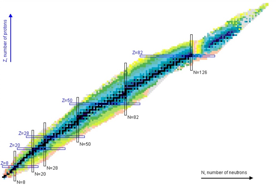
Z = Number of Protons = Vertical Axis N = Number of Neutrons = Horizontal Axis
Reference: http://www.nndc.bnl.gov/chart/
The methodology of fill of a given energy level position for a Proton or Neutron for a given nucleus of interest is completely independent of how previous Protons or Neutrons filled their respective energy level positions. The methodology of fill is only dependent upon the potential energy function for that nucleus (the kinetic energy function remains the same for all nuclei). Therefore, if the nucleus of interest has spherical symmetry, then the potential energy function will be a function proportional to 1/r. Somewhere between the magic number of 28 for the Fourth Energy Level for Protons and Neutrons in the nucleus and the magic number of 50 for the Fifth Energy Level of Protons and Neutrons in the nucleus the nucleus becomes spherical in shape. When the number of Protons and Neutrons in the Nucleus each number 50 or greater, the classical shape of the Nucleus is a near perfect sphere. Proton Energy Levels Six through Eight fill in identical manner to Electron Energy Levels Six through Eight. Neutron Energy Level Six fills in identical manner to Electron Energy Level Six. The deviation for Neutron Energy Levels above Level Six can be accounted for by the need to raise the Nuclear Gravitation Field intensity to overcome the rising Coulombic Repulsion Force tending to break the Nucleus apart. It is safe to conclude that when the classical shape of the Nucleus is a near perfect sphere, then the Nuclear Gravitation Field Potential Function is proportional to 1/r2 and consistent with Newton’s Law of Gravity.
Nuclear Gravitation Field Required to Overcome Nuclear Electric Field Repulsion
Nuclear Fusion: The Proton-Proton-Chain
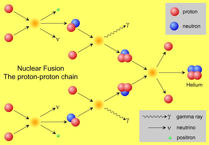
Assume we will initiate the first step to fusing Hydrogen to Helium in the same manner that takes place within the interior of our Sun. In this case, we must bring two protons in contact with one another. In order to accomplish this, we must overcome the like charge Coulombic repulsion of each of the protons – the Nuclear Electric Field established by each proton. Let’s determine the minimum intensity of the Strong Nuclear Force – the minimum intensity of the Nuclear Gravitation Field required to overcome the Nuclear Electric Field repulsive force present at the surface of the Proton in order to bring the second Proton into contact with our Proton. The radius, r, of each Proton is equal to 1.20 x 10⁻¹⁵ meter, therefore, the distance between the centers of each Proton in contact is twice the radius of each Proton or 2.40 x 10⁻¹⁵ meter. The equation for Force between electrically charged particles is as follows:
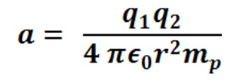
q1 is the charge of the first Proton; q2 is the charge of second Proton placed in contact with the first Proton to establish the repulsive force, F; ∈0 is the permittivity of the Electric Field in free space; and r is the distance between the centers of each of the Protons. We also know that the classical physics calculation for force acting on a body, in this case the Nuclear Electric Field of the first Proton acting upon the second Proton, is as follows:
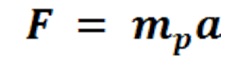
Where F is Force, mp is the mass of the second Proton being acted upon by the Nuclear Electric Field of the first Proton, and a is the acceleration of the second Proton. In order for both Protons to remain in contact with one another, the Strong Nuclear Force – Nuclear Gravitation Field force holding the second Proton to the first Proton - must be, at a minimum, equal and opposite to the Nuclear Electric Field repulsion force repelling the second Proton from the first Proton. If the forces are equal and opposite, then the acceleration fields associated with those forces must be equal and opposite. Each field is acting upon the second Proton with a mass mp. Using both equations, above, the acceleration sensed by the second Proton being repelled by the first Proton can be determined by solving for acceleration, a, as follows:
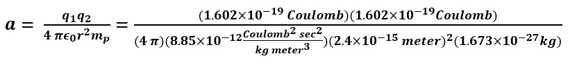
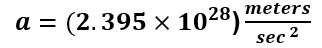
Divide the acceleration field, a, by the acceleration of gravity on Earth, 9.81 meters/sec2, to obtain the acceleration field in g’s.
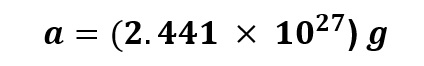
TThe value of acceleration, a, represents the repulsive Nuclear Electric Field established by the first Proton acting upon the second Proton of interest. In order to overcome the Nuclear Electric Field repulsion of the second Proton from the first Proton, the minimum required acceleration field required by the Strong Nuclear Force – the Nuclear Gravitation Field – to hold the second Proton next to the first Proton is 2.441 x 1027g.
In order to determine whether or not the Nuclear Gravitation Field at the surface of the nucleus has an intensity great enough to result in observable General Relativistic effects, one must compare the Nuclear Gravitation Field at the surface of the nucleus to the gravitational field in the vicinity of the Sun’s surface and in the vicinity of the surface of a Neutron Star. Gravitational fields in the vicinity of stars are more than intense enough for significant General Relativistic effects to be observed. The Neutron Star was selected as one of the cases to study because the density of the nucleus, which is made up of protons and neutrons, is very close to the density of a Neutron Star. A Neutron Star typically contains the mass approximately that of our Sun, however, the matter is concentrated into a spherical volume with a diameter of about 10 miles or 16 kilometers. The radius of a Neutron star is about 5 miles or 8 kilometers. The following figure illustrates the relative size of the Earth to the size of a White Dwarf star and a Neutron star.
Comparative Sizes of the Earth,
a Typical White Dwarf Star,
and a Typical Neutron Star
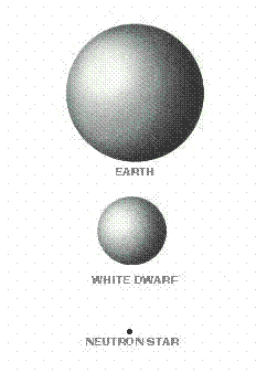
Reference: “The Life and Death of Stars,” by Donald A. Cooke, Page 131, Figure 8.12
Let’s determine the gravitational field at the surface of a Neutron Star. The Neutron Star is assumed to contain the same mass as the Sun, therefore, the mass of the Neutron Star, “MNeutron Star,” is equal to 1.99×1030 kg. The Neutron Star’s radius, which is defined as “RNeutron Star,” is about 5 miles equal to about 8 km or 8.0×10
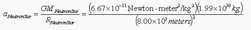
aNeutron Star = 2.07×10¹²N-kg-1 = 2.07×10¹² meters/second2
To determine the “g-force” at the Neutron Star’s surface, the gravitational field of the Neutron Star must be normalized relative to Earth’s gravitational field in the same manner used to calculate the g-force at the Sun’s surface. Earth’s gravitational field is 1g. The ratio of the acceleration of gravity on the Neutron Star’s surface to the acceleration of gravity on the Earth’s surface represents the g-force on the Neutron Star’s surface. The g-force on the Neutron Star’s surface is calculated as follows:
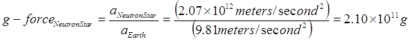
Albert Einstein’s General Relativity Theory was confirmed in 1919 when a total eclipse of the Sun occurred. With the Sun being blocked out by the Moon, a star directly behind the Sun could be seen on either side of the Sun due to the acceleration of light around the Sun. The gravitational field of the Sun at 27.8g can warp or bend Space-Time. The gravitational field of a Neutron Star, at 2.10×10¹¹g, has an intensity over 7.5 billion times greater than the Sun’s gravitational field. The Neutron Star’s gravitational field will result in substantial “Space-Time Compression.” The minimum gravitational field intensity at the surface of the Proton was calculated to be 2.441 x 1027g, a value over 16 decades more intense than the value calculated for a Neutron Star. The General Relativistic effects next to the Nucleus of the Atom must be considered.
General Relativity and Space-Time Compression
Space-Time Compression:
What is Space-Time Compression and how is it related to Special Relativity and General Relativity? Space-Time Compression is the relativistic effect of reducing the measured distance and light travel-time between two points in space as a result of the presence of either:
Two or more inertial reference frames where relativistic velocities (velocities of a significant fraction of the velocity of light) between the reference frames are involved – Special Relativity. A spacecraft traveling at 0.98c (98% of the velocity of light) relative to Earth is an example of two relativistic inertial reference frames.
- Accelerated reference frames defined by either the physical acceleration, or change in velocity, of an object of interest relative to a point of reference in Space-Time in the presence of an acceleration field – General Relativity. An example of an accelerated reference frame is that of the Sun’s gravitational field, equal to 27.8g, near the Solar surface. Space-Time Compression occurs because of the invariance of the measured, or observed, velocity of light: 186,300 miles/sec = 299,750 km/sec, independent what inertial or accelerated reference frame the observer exists within or externally observes from. Inertial Reference Frames:
The methodology for the filling of Proton and Neutron Energy Levels in the Nucleus of the Atom indicates that the Strong Nuclear Force field propagates omnidirectional outward to infinity from the Nucleus. When the Nucleus has a sufficient number of nucleons present to form a near perfect sphere, the Strong Nuclear Force field propagates outward omnidirectional to infinity with spherical symmetry resulting in the Gravitational Potential Field following a 1/r2 function. Therefore, the outward propagation of the Strong Nuclear Force field is consistent with Newton’s Law of Gravity.
The observed virtual disappearance of the Strong Nuclear Force at the surface of the Nucleus is a result of extreme Space-Time Compression. This General Relativistic effect can only occur if the Strong Nuclear Force field is Gravity. Only Gravity fields can accelerate light, electric fields, or magnetic fields to produce Space-Time Compression. Gravity propagates based upon Uncompressed Space-Time; Light, Electric Fields, and Magnetic Fields propagate based upon Compressed Space-Time.
Neutrons are required to be added to the Nucleus to raise the strength to the Strong Nuclear Force to overcome the rising Coulombic Repulsion Force of the Protons as Protons are added to the Nucleus. Space-Time Compression within the Nucleus results in the Nuclear Gravitation Field rising slower than the Nuclear Electric Field as Protons are added to the Nucleus. The Nuclear Gravitation Field propagates outward within the Nucleus based upon Uncompressed Space-Time so its intensity rises slower / drops faster than the Nuclear Electric Field propagating outward through the Nucleus.
The Strong Nuclear Force appears to saturate as Protons and Neutrons are added to the Nucleus - Element 83, Bismuth-209, is the largest known Nucleus that is stable. Space-Time Compression within the Nucleus results in the Nuclear Gravitation Field rising slower than the Nuclear Electric Field as Protons are added to the Nucleus. The Nuclear Gravitation Field propagates outward within the Nucleus based upon Uncompressed Space-Time so its intensity rises slower / drops faster than the Nuclear Electric Field propagating outward through the Nucleus. The Nuclear Electric Field is approaching the strength of the Nuclear Gravitation Field, therefore, the Elements beyond Bismuth are radioactive.
- U.S. Naval Nuclear Power School in Orlando Florida, from September 1977 to March 1978 - Class 7709.
Naval Nuclear Power School is a six-month intense curriculum of applied mathematics, chemistry, thermodynamics, mechanical engineering, electrical engineering, and pressurized water reactor theory, design, and operation of a Naval Nuclear Propulsion Plant.
United States Naval Nuclear Power School
Orlando, Florida - U.S Naval Nuclear Propulsion Prototype Training Unit training at the Naval Reactors Facility on the Idaho National Engineering Laboratory Site about 60 miles west of Idaho Falls, Idaho, from April 1978 to September 1978 - Class 7709.
Naval Nuclear Prototype Training is a six-month intense training on an operating reactor plant similar to those on Nuclear Powered Surface Ships and Submarines. I qualified as an Engineering Officer of the Watch (EOOW) on the S1W Reactor Plant Prototype for the First Nuclear Fast Attack Submarine - U.S.S. Nautilus (SSN-571). - U.S. Naval Submarine Officer Basic Course at the Naval Submarine Base, Groton, Connecticut, from October 1978 to January 1979.
Submarine Officer Basic Course is three-months of training to introduce the student to submarine underway operations and the non-nuclear systems supporting those operations. - Brunswick Nuclear Plant: A two-unit site, each is a General Electric Boiling Water Reactor
- Catawba Nuclear Station: A two-unit site, each is a Westinghouse 4-Loop Pressurized Water Reactor
- H. B. Robinson Nuclear Plant: A single unit site with a Westinghouse 3-Loop Pressurized Water Reactor
- McGuire Nuclear Station: A two-unit site, each is a Westinghouse 4-Loop Pressurized Water Reactor
- Oconee Nuclear Station: A three-unit site, each is a Babcock and Wilcox 2-Loop Once-Through Steam Generator Pressurized Water Reactor
- Shearon-Harris Nuclear Plant: A single unit site with a Westinghouse 3-Loop Pressurised Water Reactor
- Gravity Warp Drive Home Page
- Nuclear Gravitation Field Theory
- History of My Research and Development of the Nuclear Gravitation Field Theory
- “The Zeta Reticuli Incident” by Terence Dickinson
- Supporting Information for the Nuclear Gravitation Field Theory
- Government Scientist Goes Public
- The Physics of Star Trek and Subspace Communication: Science Fiction or Science Fact?
- “Sport Model” Flying Disc Operational Specifications
- Design and Operation of the “Sport Model” Flying Disc Anti-Matter Reactor
- Element 115
- Bob Lazar’s Gravity Generator
- United States Patent Number 3,626,605: “Method and Apparatus for Generating a Secondary Gravitational Force Field”
- United States Patent Number 3,626,606: “Method and Apparatus for Generating a Dynamic Force Field”
- V. V. Roschin and S. M. Godin: “Verification of the Searl Effect”
- Constellation: Reticulum
- Reticulan Extraterrestrial Biological Entity
- Zeta 2 Reticuli: Home System of the Greys?
- UFO Encounter and Time Backs Up
- UFO Testimonies by Astronauts and Cosmonauts and UFO Comments by Presidents and Top U.S. Government Officials
- Pushing the Limits of the Periodic Table
- General Relativity
- Rethinking Relativity
- The Speed of Gravity - What the Experiments Say
- Negative Gravity
- The Bermuda Triangle: Space-Time Warps
- The Wright Brothers
- Favorite Quotes from Famous People
- Sponsors of This Website
- Romans Road to Eternal Life In Jesus Christ
One way to quantitatively observe the Space-Time compression effect is to look at the blue right triangle within a quarter circle of unity radius (radius, r = 1) displayed in the figure, below. The hypotenuse of the triangle is the side of the blue triangle starting from the center of the circle moving diagonally upward and to the right with a length unity, or 1, and equal to the radius of the quarter circle. The hypotenuse of the blue right triangle represents the velocity of light, c, as a fraction of the velocity of light, c, or c/c = 1.
Trigonometric Identities and Relationship to Relativity
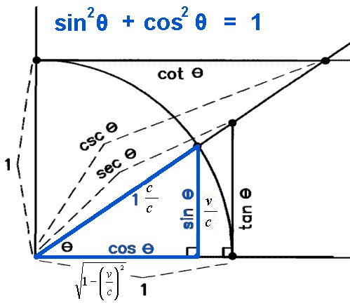
The vertical side of the blue right triangle is the ratio of the velocity of the spacecraft to that of the velocity of light, or v/c and is the “opposite side” from the angle formed by the hypotenuse of the blue right triangle, or the radius of the quarter circle, and the horizontal side of the blue right triangle. That angle is represented by the Greek letter θ (Theta). The angle θ spans from 0° to 90°. The length of the vertical side of the blue right triangle is equal to sinθ, therefore, v/c = sinθ. The horizontal side of the blue right triangle represents the amount of Space-Time Compression that reduces the distance between two points in Space-Time (length contraction) and reduces the time it takes light to travel between the two points (time dilation) based on the velocity of the spacecraft relative to the velocity of light. The length of the horizontal side of the blue right triangle is equal to cosθ. Using the Pythagorean Theorem, we can solve for cosθ.
sin2θ + cos2θ = 1
v/c = sinθ
Substitute v/c for sinθ, then solve for cosθ
(v/c)2 + cos2θ = 1
cos2θ = 1 – (v/c)2
cosθ = [1 – (v/c)2]1/2
1/cosθ = secθ = 1/[1 – (v/c)2]1/2 = “Space-Time Compression Factor”
The “Space-Time Compression Factor” is the multiplicative inverse of the value of length of the horizontal side of the blue right triangle equal to 1/cosθ, or secθ, and is designated by the Greek Letter γ (gamma). The length contraction and time dilation can be determined by solving for the length of the horizontal side of the triangle using the Pythagorean Theorem. Therefore, the distance between the Earth and the star of interest 10 light-years away as measured by the observer in the spacecraft moving at a velocity, v, is defined as follows:
d = d0 [1 – (v/c)2]1/2
Where d0 is the measured distance to the star of interest in “Normal Space-Time” or “Uncompressed Space-Time” as measured by the observer on the Earth and d is the “Compressed Space-Time” distance (or length contracted distance) as measured by the observer in the spacecraft moving at a velocity, v. The reduction of time for light to travel the distance between the star of interest and spacecraft in the vicinity of Earth is affected in the same manner by “Space-Time Compression.” Einstein noted the equivalence of space and time, hence the term Space-Time is used. The relationship of space and time is as follows:
d = ct
d represents distance, c represents the velocity of light, and t represents elapsed time. Substituting ct for d and ct0 for d0, the distance compression equation can become a time dilation equation.
ct = ct0 [1 – (v/c)2] Therefore: t = t0 [1 – (v/c)2]1/2 The following table provides the values for length contraction and “Space-Time Compression Factor” as a function of velocity relative to the velocity of light, c = 299,750 km/sec = 186,300 miles/sec. As indicated in the table, above, measured velocities do not contribute significantly to the “Space-Time Compression” effect unless the measured velocity is a significant fraction of the the velocity of light, c. At a measured velocity of 0.995c, the “Space-Time Compression Factor” is just above 10 and at a measured velocity of 0.999c, the “Space-Time Compression Factor” is just under 22.4. Table “Velocity and Space-Time Compression” introduces the concept of effective velocity. When the spacecraft is traveling at a measured velocity of 0.707c, the effective velocity, veff, of the spacecraft is 1.000c or the speed of light, c. Although the spacecraft only has a measured velocity as 0.707c, the length contraction along the line of travel is reduced to 0.707 (or 70.7%) of the original distance (which represents a “Space-Time Compression Factor” equal to 1.414), therefore, the time to travel the uncompressed distance (which is a known quantity) is equal to the time it would take light to travel the uncompressed distance. The evaluation, above, discusses Space-Time Compression as a function of a constant relativistic velocity, therefore is an evaluation of a inertial reference frame. General Relativity includes the evaluation of accelerated reference frames. Gravity fields establish accelerated reference frames because gravity accelerates light, electric fields, and magnetic fields. Therefore, gravity fields generate the Compressed Space-Time due to the acceleration of light, electric fields, and magnetic fields. Since the speed of light will always be measured as propagating at a constant speed of 2.9975 x 10⁸ meters/sec, the distance traveled is reduced by the Space-Time Compression Factor. Light, Electric Fields, and Magnetic Fields propagate based upon Compressed Space-Time. We determined that the minimum Nuclear Gravitation Field acceleration has to be at least 2.441 x 1027g, therefore, the effects of General Relativity must be considered. Gravity fields propagate based upon Uncompressed Space-Time. In order to “see” or “measure” the Nuclear Gravitation Field propagating outward from the Nucleus omnidirectional in spherical symmetry dropping in intensity 1/r2 consistent with Newton’s Law of Gravity, we would have to measure the field intensity in Uncompressed Space-Time. However, we live in the Compressed Space-Time reference frame, therefore, we see events in Compressed Space-Time. As previously discussed, gravity fields generate the Compressed Space-Time due to the acceleration of light, electric fields, and magnetic fields. Light, Electric Fields, and Magnetic Fields propagate based upon Compressed Space-Time. Table “Accelerated Reference Frame Space-Time Compression Due to Gravity Field,” below, determines the Uncompressed Space-Time acceleration of light as a function of the intensity of various gravity fields, determines the reduction in the distance traveled by light as observed in Compressed Space-Time, and the resulting Space-Time Compression Factors. Let’s assume the gravitational field next to the nucleus of the atom was equal to 2.9975 x 10⁸ meters/sec2. If light was subjected to this acceleration field, in one second the speed of light would be doubled to 5.9950 x 10⁸ meters/sec equal to the speed of light in Uncompressed Space-Time. Since the speed of light in free space is invariant with respect to the reference frame of the observer, the speed of light remains at 2.9975 x 10⁸ meters/sec. Therefore, the distance traveled by light in Compressed Space-Time must be reduced to half the Uncompressed Space-Time distance as indicated by the first entry highlighted in red in Table, “Accelerated Reference Frame Space-Time Compression Due to Gravity Field,” below. In accordance with the article “The Speed of Gravity – What the Experiments Say” by the late Associate Professor Tom Van Flandern, gravity propagates at least 20 billion times faster than light and may propagate instantaneously. No term in the force equation for Newton’s Law of Gravity provides a speed of gravity field propagation. Gravity has a value of intensity at a given distance from the mass of interest. The only time dependent function in Newton’s Law of Gravity is the gravity acceleration field acting upon a mass of interest at a given position in space, therefore, it is assumed that gravity propagates instantaneously. Final Uncompressed Space-Time velocity of light after one second can be calculated in a specific gravitational field if the units used are consistent for velocity and acceleration – in this case meters/second and meters/second2. From Table “Accelerated Reference Frame Space-Time Compression Due to Gravity Field,” the Space-Time Compressed distance that light travels, at five significant digits, is zero distance for any gravity field acceleration field greater than 1.00 x 10¹³g. The minimum gravitational acceleration field required to overcome like charge Coulombic Repulsion of two Protons in contact is 2.441 x 1027g results in Space-Time Compression to zero distance because the Space-Time Compression Factor equals 7.99873 x 10¹⁹ as indicated by the second entry highlighted in red in Table “Accelerated Reference Frame Space-Time Compression Due to Gravity Field.” The characteristic “vanishing” of the Strong Nuclear Force at the surface of the Nucleus can only occur if the Strong Nuclear Force accelerates light, therefore, the Strong Nuclear Force must be Gravity. The Nuclear Gravitation Field next to the Proton is much greater than the classical physics calculated gravitational field near a Neutron Star or Black Hole. The Nuclear Gravitation Field intensity drops about 19 decades just outside the Nucleus before the gravitational field can be “seen” or “measured” propagating outward from the Nucleus because we observe the Nuclear Gravitation Field in a Compressed Space-Time reference frame. The Space-Time Compression occurring next to the nucleus is so significant that if we could view the atom in Uncompressed Space Time, the Electron Cloud exit would be on the order of a half meter away from the Nucleus. Let’s assume that the Strong Nuclear Force from a single Proton provides the minimum gravitational acceleration to overcome the like charge Coulombic repulsion of a second Proton. The gravitational acceleration field of the Proton at its surface is 2.395 x 1028 meters/second2. The diameter of the Proton is 2.40 x 10⁻¹⁵ meter, therefore, the radius of the Proton is 1.20 x 10⁻¹⁵ meter. The Proton Strong Nuclear Force Field – the Nuclear Gravitation Field intensity – at a distance of 1.20 x 10⁻¹⁵ meter from the center of the Proton is 2.395 x 1028 meters/second2. Using Newton’s Law of Gravity, calculate the distance the Proton gravitational field must propagate outward in Uncompressed Space-Time before the intensity of the gravitational field has dropped sufficiently to result in a measurable outward propagation of the Proton gravitational field from the Proton in Compressed Space-Time. Newton’s Law of Gravity is as follows: The Proton’s gravitational field propagates outward with spherical symmetry, therefore, the Proton gravitational field intensity will drop off proportional to 1/r2 where the initial gravitational field intensity at a distance 1.20 x10⁻¹⁵ meter is 2.395 x 1028 meters/second2. Determine the Proton gravitational field at various distances from the Proton surface in Uncompressed Space-Time using the Newton’s Law of Gravity 1/r2 proportionality. Starting at the Proton surface with a gravitational field of 2.395 x 1028 meters/second2, calculate the Gravitational Field and the Speed of Light in Uncompressed Space-Time at various Uncompressed Space-Time distances from the Proton surface to determine the Space-Time Compression Factors and the equivalent Compressed Space-Time distances from the Proton surface. Table “Proton Gravity Field Propagation in Uncompressed Space-Time and Compressed Space-Time,” below, provides the calculation results. As indicated in Table “Proton Gravity Field Propagation in Uncompressed Space-Time and Compressed Space-Time,” above, the Proton gravitational field just begins to propagate outward from the Proton surface as observed in Compressed Space-Time at three significant digits at a gravitational acceleration field of 8.621 x 10¹¹ meters/second2. The Proton gravitational field in Compressed Space-Time must drop in intensity by over 19 decades, from 2.395 x 1028 meters/second2 to 1.379 x 10 As we see the Hydrogen Atom in our Compressed Space-Time reference frame, the diameter of the Hydrogen Atom is on the order of 1.00 x 10⁻¹⁰ meter, therefore, the radius of the Hydrogen atom is on the order of 5.00 x 10⁻¹¹ meter. The Uncompressed Space-Time distance from the Proton is 0.5 meter and the quantized Nuclear Gravitation Field intensity is 1.379 x 10⁻¹ meters/sec2 equal to 1.406 x 10⁻²g, at a Compressed Space-Time distance of 6.12 x 10⁻¹¹ meter, a relatively feeble gravitational field, as highlighted in the second red entry of Table “Proton Gravity Field Propagation in Uncompressed Space-Time and Compressed Space-Time,” above. However, this Nuclear Gravitation Field appears to be much too large to be the gravity we observe outside the Electron Cloud of the Hydrogen Atom. The intensity of Quantized Nuclear Gravitation Field is associated with specific, discrete, energy levels, therefore, has a value decades larger than the average gravity measured outside the Electron Cloud and requires evaluation. The Nuclear Gravitation Field must be stronger than the Nuclear Electric Field at the Nuclear Surface in order to hold the nucleons in the Nucleus together. The average Nuclear Gravitation Field intensity propagating through the outer Electron Cloud is less than 1.0 x 10⁻¹² the intensity of the Nuclear Electric Field propagating through the outer Electron Cloud. The General Relativistic effect of Space-Time Compression is the reason for the vertical drop in Nuclear Gravitation Field intensity just outside the nucleus. Nuclear Gravitation Field and The Nuclear Gravitation Field is stronger than the Nuclear Electric Field at the Nuclear Surface in order to hold the nucleons in the Nucleus together. Nuclear Gravitation Field intensity outside the Electron cloud is less than 1.0 x 10⁻³⁵ the intensity of Nuclear Electric Field outside the Electron cloud. Space-Time Compression is directly proportional to the intensity of the Nuclear Gravitation Field. Quantized gravity will be on the order of 1.0 x 10⁸ to 1.0 x 10⁹ times greater than the average gravity measured outside the electron cloud of the Atom. Therefore, gravity leaving the electron cloud will be 1.0 x 10⁻¹⁶g or less. Quantized Gravity is analogous to the Classical Physics and Quantum Mechanical evaluation of Light and how the Photo-Electric Effect occurs. In order to compare Classical Physics to Quantum Mechanics, the energy of light shining on a surface must be assumed to be a continuous distribution. In other words, light energy is assumed neither to be discrete nor quantized. Based upon that assumption, the amount of energy available to be absorbed by an electron can be determined. That calculated value will then be compared to the results of Millikan’s “Photoelectric Effect” experiments. For this calculation, a 100 watt (Joules/second) orange light source with a wavelength of 6000 Angstroms is directed onto a square plate of Sodium 0.1 meter by 0.1 meter. The surface area of the square Sodium plate is 0.01 meter2. It is assumed that all the light emitting from the orange light source is directed onto the Sodium plate. The atomic radius of the neutral Sodium atom is 2.23 Angstroms which is equal to 2.23×10⁻¹⁰ meter. The diameter of the Sodium atom is twice the radius or 4.46 Angstroms equal to 4.46×10⁻¹⁰ meter. It now must be determined how many Sodium atoms can fill the square surface of the Sodium plate assuming only the top layer of Sodium atoms (one Sodium atom deep). Although the Sodium atoms are spheres, this calculation will assume that they are square. The side of the “square Sodium atom” has the same length as the diameter of the spherical atom. A spherical atom of Sodium will fit into each of the theoretical “square Sodium atoms” that make up the top layer of Sodium atoms on the square plate. Therefore, each Sodium atom will take up the following surface area on the plate: Area of Sodium Atom = (4.46×10⁻¹⁰ meter)×(4.46×10⁻¹⁰ meter) = 1.989×10⁻¹⁹ meter2 Number of Sodium Atoms on Surface of Plate = Area of Plate divided by Area of Sodium Atom Number of Sodium Atoms on Surface of Plate = (0.01 meter2)/(1.989×10-19 meter2) Number of Sodium Atoms on Surface of Plate = 5.027×10¹⁶ Sodium
Atoms In one second, the Sodium plate surface absorbs 100 Joules of energy. 1 electron volt (eV) is equal to 1.6022×10⁻¹⁹ Joules. The next step is to calculate the amount of energy imparted to one Sodium atom in eV assuming a continuous even distribution of light energy across the Sodium plate. The intent here is to perform a comparison of the values of the classical electron absorption energy to the Quantum Mechanical electron absorbed energy as provided in Figure “Sodium Plate Photo-Electric Effect Results,” below. Photo-Electric Effect on Sodium Plate Sodium Plate Photo-Electric Effect Results Reference: http://hyperphysics.phy-astr.gsu.edu/hbase/mod2.html Energy Imparted to 1 Sodium Atom (ENa) = Total Energy Imparted to Plate divided by Number of Sodium Atoms = 5.027 x 10¹⁶ Na-atoms Each Sodium atom is receiving 1.242×10⁴ eV of energy each second. The light is only illuminating one side of the Sodium atom because it is coming from one direction, therefore, as the spherical Sodium atom is considered, half the surface area of the Sodium atom is illuminated by the light. The total surface area of a spherical Sodium Atom is calculated as follows: The illuminated portion of the sphere of the Sodium atom is equal to half the value calculated, above, or 3.124×10⁻¹⁹ meter2. In actuality, from a classical point of view, the size of the Sodium Atom is not important or required to determine how much light energy the electron will receive from the from the light source based on classical physics. The size and exposed surface area of the electron is all that is required to complete this calculation. In this calculation it is assumed that the density of an electron is the same as the density of a proton or neutron. The mass of a proton, neutron, or electron is proportional to the cube of its radius or its diameter. The surface area of either the proton, the neutron, or the electron is proportional to the cube root of its volume squared. The surface area of the electron, then, should be proportional to the surface area of a proton or neutron by the ratio of its mass to the mass of a proton or neutron to the 2/3 power. The diameter of a proton or neutron is about 1.0×10⁻¹⁵ meter. The radius of a proton or neutron is equal to half the diameter or about 0.5×10⁻¹⁵ meter. The total surface area of either a proton or neutron is calculated below: Since the light is shining from one direction, the light only illuminates half of the surface area of either a proton or neutron. Therefore, the illuminated surface area of a proton or neutron is equal to 1.571×10⁻³⁰ meter2. The electron mass is only 1/1840 that of the proton or neutron. Therefore, the surface area of an electron will be equal to the surface area of a proton or neutron multiplied by the cube root of 1/1840 squared. The surface area of an electron can be calculated based upon the surface area of a proton or neutron (nucleon) as follows: Asurface-electron = 2.092×10⁻³² meter2 Since the light is shining from one direction, the light only illuminates half of the surface area of the electron. Therefore, the illuminated surface area of the electron is equal to 1.046×10⁻³² meter2. The calculated amount of energy by the classical physics illumination from the light source received by the Sodium’s electron is as follows: The Classical Physics analysis predicts the electron only receives 4.163×10⁻¹⁰ eV of light energy per second. The amount of energy required to liberate an electron from the Sodium atom is on the order of 0.5 eV. The Classical Physics analysis result indicates that it is impossible for the photoelectric effect to ever take place. Quantum Mechanics predicts that the electron can absorb energies on the order of 0.5 eV or greater and can be liberated from the Sodium atom because the incoming light energy propagates in discrete packets or quanta of energy rather than as a continuous distribution of energy. The vast difference in magnitude of the energy that the electron would absorb based upon Classical Physics to the amount of the energy the electron will absorb by Quantum Mechanics is extremely important. It is quite reasonable to assume that this significant relative difference in magnitude of field intensity can also apply to the intensity of the Nuclear Gravitation Field. The Nuclear Gravitation Field would be much more intense if it was a discrete function rather than a continuous function. Figure “Sodium Plate Photo-Electric Effect Results,” above, states the electron Kinetic Energy is about 0.5 eV when it absorbs light at a wavelength of 6000 Angstroms. The electron must absorb a minimum amount of “Ionization Energy” to remove it from the Sodium atom before it obtains any Kinetic Energy. To be conservative, this calculation assumes the Ionization Energy of the electron in the 3s orbital of the Sodium atom to be equal to zero. The ratio of the quantized energy absorbed by the electron versus the classical calculated energy absorbed by the electron is as follows: Let’s determine the classical physics gravitational field of the Proton at the surface of the Proton. Let’s determine the classical gravity field for the Proton outside the Hydrogen Atom Electron Cloud assuming the Electron Cloud radius is equal to 5.00 x 10⁻¹¹ meter. The ratio of the amount of energy absorbed by the electron via Quantized Light, assuming the principles of Quantum Mechanics, versus the amount of energy which would have been absorbed by the electron, assuming Classical Physics, is on the order of 1.201×10⁹ times greater or over a billion times greater. It is expected that Quantized Gravity associated with the nuclear spectral line energy levels would behave in a similar manner to Quantized Light associated with spectral lines electron energy levels. However, the ratio of Quantized Gravity to average gravity would be expected to be on the order of 1,000,000 times larger than the ratio for Quantized Light energy to average light energy. The energy levels in the Nucleus are on the order of MeV (millions of electron volts) and the energy levels of the electrons in energy levels around the Nucleus are on the order of eV (electron volts). Since the nuclear energy levels are shorter in wavelength by a factor of 1 million, Quantized Gravity is expected to have an intensity on the order of 1.00 x 10¹⁵ to 1.00 x 10¹⁶ times greater than the average gravity measured outside the Electron Cloud of the Hydrogen Atom. The higher the energy associated with an energy level, the narrower the bandwidth, the lower the energy associated with an energy level, the broader the bandwidth. As previously calculated and provided in Table “Proton Gravity Field Propagation in Uncompressed Space-Time and Compressed Space-Time,” above, the Quantized Nuclear Gravitation Field intensity of a Proton is 1.379 x 10⁻¹ meters/sec2 equal to 1.406 x 10⁻²g, at a Compressed Space-Time distance of 6.12 x 10⁻¹¹ meter. The classical physics Proton gravity field at the Electron Cloud exit was calculated to be 4.550 x 10⁻¹⁸g. The ratio of Quantized Gravity to average gravity is calculated to be 3.090 x 10¹⁵ times larger than the ratio of Quantized Light energy to average light energy. This result falls within the expected range of 1.00 x 10¹⁵ to 1.00 x 10¹⁶ stated above. Therefore, the average gravity that would be measured outside the Hydrogen Atom Electron cloud would be consistent with the calculated Quantized Proton Nuclear Gravitation Field outside the Electron Cloud. Several properties of the Strong Nuclear Force are observed specifically because the Strong Nuclear Force is Gravity. The virtual vanishing of the Strong Nuclear Force just outside the Nuclear Surface is the primary indicator the Strong Nuclear Force is Gravity because of the intense Space-Time Compression taking place. The addition of Neutrons to the Nucleus to boost the Strong Nuclear Force intensity to maintain its intensity above the Nuclear Electric Field intensity within the Nucleus and hold the Nucleus together is directly related to the General Relativistic effect of Gravity. If the Strong Nuclear Force had nothing to do with Gravity, no such accelerated field would be produced within the Nucleus affecting the propagation of Light, Electric Fields, or Magnetic Fields and Space-Time Compression would be non-existent. Without Space-Time Compression present within the Nucleus of the atom, would there be any need for Neutrons? The observed stability curve for Nuclei require about a 1 to 1 Neutron to Proton ratio for light Nuclei and require about a 3 to 2 Neutron to Proton ratio for heavy Nuclei. The Strong Nuclear Force (Gravity) propagates based upon Uncompressed Space-Time within and outside the Nucleus and the Nuclear Electric Field propagates based upon Compressed Space-Time within and outside the Nucleus. The Strong Nuclear Force is the strongest field within the atom and is significantly stronger than the Nuclear Electric Field produced by the Protons in the Nucleus that would, otherwise, tend to tear the Nucleus apart because of the same electric charge (Coulombic) repulsion of each of the Protons. If the Strong Nuclear Force had nothing to do with Gravity, then the Strong Nuclear Force would continue to rise in intensity and remain more intense than the Nuclear Electric Field. There would be no need for Neutrons in the Nucleus because Protons connected to one another would always provide a sufficient Strong Nuclear Force to overcome Coulombic repulson and hold the Nucleus together. There would be no limit to the size of a Nucleus or how large a number a stable Element could be. The Strong Nuclear Force appears to saturate and be short ranged because the known Elements beyond Element 83, Bismuth-209, are radioactive. In order to boost the strength of the Strong Nuclear Force, Neutrons must be added to the Nucleus. For the lighter Nuclei, the ratio of Neutrons to Protons is 1 to 1. For the heavier Nuclei, the ratio of Neutrons to Protons is about 3 to 2. Refer to the Chart of the Nuclides, above. The Nuclear Gravitation Field loses its intensity because the Nuclear Gravitation Field propagates outward based upon Uncompressed Space-Time. The Nucleus exists in the same Compressed Space-Time Reference Frame that we, as observers, exist. Nuclear Gravitation and Electric Fields Within the Nucleus Let’s assume the Nucleus has a constant homogeneous mass density and constant homogeneous charge density for simplicity of calculations. Let’s determine the Strong Nuclear Force acceleration profile without Space-Time Compression and with Space-Time Compression within the Nucleus. Let’s determine the acceleration field for the Nuclear Electric Field within the Nucleus. R represents the radius of the Nucleus. p r represents the variable radial position of a Proton being evaluated between the Nuclear Center and the outer radius, R, of the Nucleus, in order to determine the acceleration field profiles. Determination of Nuclear Gravitational Field acceleration, gIN, as a function of internal distance from the Center of the Nucleus, r. Mass, M, is equal to constant mass density times Volume, ρMass x VIN, as a function of r, radial distance from Center of Nucleus. Therefore, the gravitational acceleration inside the Nucleus, gIN, is proportional to r. The mass contributing to gIN is only the mass from Center of Nucleus to position r inside the Nucleus. However, the gIN calculated previously with linear rise relative to radial distance from the Center of Nucleus, r, is not correct because it assumes classical physics. The Gravity field internal to the Nucleus is extremely intense and the effects of General Relativity must be considered. gIN must be evaluated with the effects of Space-Time Compression occurring. Gravity propagates based upon Uncompressed Space-Time. Light, Electric Fields, and Magnetic Fields propagate based upon Compressed Space-Time. We observe the Nucleus of the Atom in our Compressed Space-Time Reference Frame. gIN must be reevaluated to see how it will behave in Compressed Space-Time. The Mass of the Nucleus as a function of density and distance from the Center of the Nucleus is based upon the Compressed Space-Time radial distance, rCST, as indicated by the equation below: The Gravity Field inside the Nucleus, gIN, must be calculated based upon Uncompressed Space-Time radial distance from the Center of the Nucleus, rUST as indicated by the equation below: Substituting the calculation value for MIN, the resulting equation for calculating gIN is as follows: rUST rises faster than rCST and the rate of rise of rUST goes up because the Gravity field intensity rises as a function of rUST resulting in rising Compressed Space-Time. gIN will no longer rise linearly, it will tend to level off as rUST and rCST rise. The figure, below, indicates the behavior of gIN-NSTC, Nuclear Internal Gravity Field - No Space-Time Compression present, and gIN-CST, Nuclear Internal Gravity Field - With Space-Time Compression present: Determination of Nuclear Electric Field acceleration, aEF-IN, as a function of internal distance from the Center of the Nucleus, r. The charge distribution inside the Nucleus contributing to aEF-IN is only the charge distribution from Center of Nucleus to position r inside the Nucleus. Therefore, the Nuclear Electric Field acceleration field inside the Nucleus, aEF-IN is proportional to r. The charge distribution inside the Nucleus contributing to aEF-IN is only the charge distribution from Center of Nucleus to position r inside the Nucleus. Figure “Nuclear Field Profiles Within the Nucleus,” below, provides the field profiles as a function of distance r from the Center of the Nucleus to the Nuclear Surface. Nuclear Gravitation Field Profiles Within the Nucleus SNF-NSTC = Strong Nuclear Force - No Space-Time Compression The profiles of the Acceleration Fields listed, above, within the Nucleus as a function of Atomic Mass are provided in Figure, “Nuclear Gravitation Field and Nuclear Electric Field at Nuclear Surface as Function of Atomic Mass,” below. Nuclear Gravitation Field and Nuclear Electric Field at Nuclear Surface as Function of Atomic Mass SNF-NSTC = Strong Nuclear Force - No Space-Time Compression The equations for the acceleration fields established by the Strong Nuclear Force and the Coulombic Repulsion Force within the Nucleus demonstrate the Strong Nuclear Force must be gravity. If the Strong Nuclear Force was not gravity, Space-Time Compression would be non-existent. Protons, alone, would always provide sufficient Strong Nuclear Force nuclear attraction field to overcome the Coulombic Repulsion generated by the Nuclear Electric Field generated by the Protons no matter how many Protons exist in the Nucleus. The Nucleus would remain stable with any number of Protons from one to infinity. The Strong Nuclear Force propagating out of the Electron Clouds of all atoms would provide such an intense attractive field that all the atoms in the universe would collapse into a black hole singularity. The strong Nuclear Electric Field propagating outward from the nucleus is neutralized by electrons orbiting the nucleus. Drop-off of SNF-WSTC results in the apparent “saturation” of the Strong Nuclear Force and has a profile appearance similar to Binding Energy per Nucleon curve as indicated by Figure “Binding Energy Per Nucleon,” below. Binding Energy Per Nucleon Reference: http://www.nndc.bnl.gov/chart/ The Lead-208 isotope (82Pb208) is a “double magic” Nucleus containing 82 Protons and 126 Neutrons. For Lead-208, 82 Protons fill Six Energy Levels and 126 Neutrons fill Seven Energy Levels. The Nuclear Gravitation Field for Lead-208 is relatively strong and Space-Time Compression next to the Nuclear Surface is very significant compared to average stable nuclei. The Lead Nucleus is also near the apparent limit where the Strong Nuclear Force is able to overcome the Coulombic Repulsion Force and remain a stable nucleus. The Bismuth-209 isotope (83Bi209) has 83 Protons and 126 Neutrons. For Bismuth-209, 82 of the 83 Protons fill Six Energy Levels and 126 Neutrons fill Seven Energy Levels. The 83rd Proton is the lone Proton in Seventh Energy Level. For all the currently known stable isotopes of Elements, the Bismuth-209 nuclear configuration is unique. There are no other stable isotopes of Elements on Earth with a similar configuration. Element 83, Bismuth-209, is the last known stable isotope listed on the Periodic Table of the Elements. All identified isotopes of Elements beyond Bismuth are radioactive indicating the Coulombic Repulsion Force has become significant enough to affect the Strong Nuclear Force ability to hold those nuclei together. Radioactive decay occurs to ultimately change the Nuclei to a stable Nucleus. The lone proton in the Seventh Energy Level of the Bismuth Nucleus is “loosely” held to the Nucleus resulting in the Nuclear Gravitation Field for Bismuth-209 being significantly weaker than the Nuclear Gravitation Field for Lead-208. The weaker Nuclear Gravitation Field for Bismuth-209 results in the Nuclear Gravitation Field undergoing a significantly lesser amount of Space-Time Compression. Therefore, the gravity field outside the electron cloud for Bismuth will be greater than what would be determined by Bismuth-209 having an atomic mass of 208.980399 amu (atomic mass units) and Lead-208 having an atomic mass of 207.976652 amu. Note that the difference in mass between Bismuth-209 and Lead-208 is 1.003747 amu. The atomic mass of the Hydrogen-1 isotope is 1.007825 amu, therefore, the mass defect to bind the 83rd proton to the Bismuth-209 Nucleus is 0.004078 amu. Cavendish Experiments can be performed to demonstrate that Bismuth-209 has a stronger gravitational field beyond that associated with its mass than the gravitational field of Lead-208. The Cavendish Experiment was used to determine G in Newton’s Law of Gravity equation: Perform the Cavendish Experiment with Lead-208 to measure its Gravitation Constant GPb. Perform the Cavendish Experiment with Bismuth-209 to measure its Gravitation Constant GBi. Compare the values of GPb and GBi to the “Universal Gravitation Constant” G = Let’s first look at Newton’s Law of Gravity and the “Universal Gravitation Constant.” The following passage was extracted from “Physics, Parts I and II,” by David Halliday and Robert Resnick, pages 348 to 349. This passage discusses Lord Cavendish's Experiment designed to measure the Universal Gravitation Constant: To determine the value of G it is necessary to measure the force of attraction between two known masses. The first accurate measurement was made by Lord Cavendish in 1798. Significant improvements were made by Poynting and Boys in the nineteenth century. The present accepted value of G is 6.6726x10⁻¹¹ Newton-meter2/kg2, accurate to about 0.0005x10⁻¹¹ Newton-meter2/kg2. In the British Engineering System this value is 3.436x10⁻⁸ lb-ft2/slug2. The constant G can be determined by the maximum deflection method illustrated in the Figure, “Cavendish Experiment,” below. Two small balls, each of mass m, are attached to the ends of a light rod. This rigid “dumbbell” is suspended, with its axis horizontal, by a fine vertical fiber. Two large balls each of mass M are placed near the ends of the dumbbell on opposite sides. When the large masses are in the positions A and B, the small masses are attracted, by the Law of Gravity, and a torque is exerted on the dumbbell rotating it counterclockwise, as viewed from above. When the large masses are in the positions A' and B', the dumbbell rotates clockwise. The fiber opposes these torques as it is twisted. The angle through which the fiber is twisted when the balls are moved from one position to the other is measured by observing the deflection of a beam of light reflected from the small mirror attached to it. If the values of each mass, the distances of the masses from one another, and the torsional constant of the fiber are known, then G can be calculated from the measured angle of twist. The force of attraction is very small so that the fiber must have an extremely small torsion constant if a detectable twist in the fiber is to be measured. The masses in the Cavendish balance of displayed in Figure, “Cavendish Experiment,” below, are, of course, not particles but extended objects. Since each of the masses are uniform spheres, they act gravitationally as though all their mass were concentrated at their centers. Because G is so small, the gravitational forces between bodies on the Earth’s surface are extremely small and can be neglected for ordinary purposes. The Cavendish Experiment
In the figure, below, a comparison of two Nuclear Gravitation Fields propagating outward from the Nuclear surface, Nuclear Gravitation Field 1 has a greater intensity than Nuclear Gravitation Field 2 at the Nuclear surface. When the effect of Space-Time Compression is considered, Nuclear Gravitation Field 1 undergoes more Space-Time Compression than Nuclear Gravitation Field 2. Therefore, Nuclear Gravitation Field 2 leaving the electron cloud of the atom will have a greater intensity than Nuclear Gravitation Field 1 outside the electron cloud of the atom. As previously noted, the Nuclear Gravitation Field for Bismuth-209 should be greater than Nuclear Gravitation Field for Lead-208 because it is significantly weaker at Nuclear surface. Comparison of Nuclear Gravitation Fields Compelling evidence that the Strong Nuclear Force and Gravity are one and the same is provided below: Strong Nuclear Force = Gravity Nuclear Gravitation Field Theory e-Book Click on either the image to the left or the hyperlink, above, to obtain the Nuclear Gravitation Field Theory e-Book. I was appointed to the United States Naval Academy on July 23, 1973, to begin my Plebe Summer training. The Plebe Indoctrination Program is implemented during Plebe Summer to the new Midshipmen 4th Class (Plebes) in like manner to Boot Camp for enlisted military inductees. The Plebe Indoctrination Program continuously applies both physical and mental pressure to determine if the new Midshipmen will be able to handle the rigors of “the heat of battle” a military officer may experience in the future. The Plebe Indoctrination Program continues for the 4th Class Midshipmen during their entire first academic year at USNA. Courses for the 4th Class Midshipman academic year include Chemistry, Calculus, Introduction to Naval Science, Introduction to Naval Engineering, and History of Sea Power. Midshipman 3rd Class “Summer Cruise” involves assigning the 3rd Class Midshipmen to U.S. Navy Warships to work and stand at sea watches as Enlisted crew members. When Midshipmen graduate from USNA, they will become Commissioned Officers and be assigned to a division with Enlisted personnel working for them. Midshipman 2nd Class Summer introduces the 2nd Class Midshipmen to their career options after graduation from USNA: Navy Pilot or Naval Flight Officer at Pensacola, Florida; U.S. Marine Corps Officer at Quantico, Virginia; Submarine Service at Groton, Connecticut; and Surface Warfare Service (Surface Warships) at Newport, Rhode Island (these were the locations I visited during the Summer of 1975 – the locations may be different today for USNA Midshipmen). Midshipman 1st Class “Summer Cruise” assigns the 1st Class Midshipmen to a U.S. Navy Warship (Surface Ship or Submarine) to “shadow” a Division Officer assigned to the ship and work and stand at sea watches as a Division Officer. The Majors Program begins during the 3rd Class Midshipman academic year and Majors are selected during the second semester of 4th Class Midshipman academic year. All Midshipmen major in Naval Engineering to prepare them to be Naval Officers assigned to a U.S. Navy Warship. The Majors Program allows a Midshipman to focus on specific areas of study. 80% of the Midshipmen must select an Engineering or Technical Major. I selected Physics as my major. Required courses for 3rd Class Midshipman academic year include Naval Ship Design and Navigation – Piloting and Celestial. Required Courses for 2nd Class Midshipman academic year include Applied Thermodynamics - Steam Plant Design and Electrical Engineering as applicable to a U.S. Navy Warship. Required Courses for 1st Class Midshipman academic year include Naval Weapons Systems and Leadership. Courses required for the Physics Major include Differential Equations, Advanced Engineering Mathematics, Physical Mechanics I and II, Electricity and Magnetism I and II, Thermal Physics, and Physics of the Atom I and II (Quantum Physics). To complete the required course hours for the Physics Major, one could select from a list of elective courses. I completed my Physics Major with Nuclear Physics and Solid State Physics. I also completed Reactor Physics I and II to learn the design and operation of a Nuclear Fission Reactor and prepare for Submarine duty. I completed the 4-year program and obtained a Bachelor of Science Degree from the United States Naval Academy in Annapolis, Maryland, on June 8, 1977. Upon receiving my degree, I obtained a Commission as an Ensign in the United States Navy. Click on each image, below, to see a larger image of my Bachelor of Science Degree, my Naval Officer Commissioning document, or larger photographs of the United States Naval Academy. Upon Commission as an Officer in the United States Navy, I continued the education required to prepare me for service in the United States Nuclear Navy Submarine Fleet. I attended and successfully completed the following schools:
Naval Nuclear Prototype Training Unit United States Naval Submarine Base Several years later after leaving the U.S. Navy while employed by Southern California Edison at the San Onofre Nuclear Generating Station I had the opportunity to further my education. I attended the University of Phoenix in San Diego, California, from January 1998 to December 2000, and obtained a Master of Science Degree in Computer Information Systems – essentially a Master of Science Degree in Business Administration with emphasis in Computer Science. I served as a Naval Officer assigned to United States Navy Nuclear Fast Attack Submarine U.S.S. Flasher (SSN-613) home ported in San Diego, California, from January 1979 through June 1982. During my sea tour aboard U.S.S. Flasher (SSN-613), I served as the Electrical Officer, the Communications and Electronic Materials Officer, the Main Propulsion Assistant to the Engineer Officer, and Assistant Operations Officer. I began my tour aboard U.S.S. Flasher at the rank of Ensign United States Navy (0-1) and completed my tour aboard U.S.S. Flasher at the rank of Lieutenant United States Navy (O-3). From November 1979 to June 1980, I participated in my first Western Pacific Deployment aboard U.S.S. Flasher. I became a Member of the Realm of the Golden Dragon when U.S.S Flasher, steaming westbound, crossed the 180th Meridian (180° West or East), also known as the International Date Line. When one crosses the International Date Line heading west, clocks are moved ahead 24 hours or one day. During the first half of the deployment, U.S.S. Flasher was originally scheduled to make a port call at Sattahip, Thailand, for Christmas 1979. However, due to the Iranian government taking hostage the United States Citizens working at the U.S. Embassy in Tehran, Iran, U.S.S. Flasher was re-directed to steam to the Indian Ocean to monitor shipping activity near the Strait of Hormuz. The trip to the Indian Ocean required U.S.S. Flasher to cross the Earth’s Equator, in the vicinity of the East Indies. Since I had never previously crossed the Equator heading south on a U.S Navy ship, I was considered a greasy, grimy, polliwog. I participated in the Shellback initiation ceremony (much like a college freshman going through an initiation to become a member of a college fraternity) and became a Certified Shellback. Click on each image, below, to see a larger image of each respective certificate. The second half of the deployment, U.S.S. Flasher participated in operations in the Western Pacific Ocean. Specific details of submarine operations performed during the deployment were highly classified. During this deployment, U.S.S. Flasher made port calls to Pearl Harbor, Hawaii; Guam; Subic Bay, Philippines; Yokosuka, Japan; and Pusan, South Korea. In June 1981 I completed all the requirements for Qualification in Submarines giving me the right to wear the Gold Dolphins with honor and become a member of a very elite group of people. For a Naval Officer to “Qualify in Submarines” he is required to qualify as Engineering Officer of the Watch (EOOW) on the Submarine Nuclear Propulsion Plant, qualify as Diving Officer of the Watch (DOOW), and qualify as Officer of the Deck (OOD) Surfaced and Submerged. Click on each image, below, to see larger images of my Submarine Qualification Certificate and the Gold Dolphins. From July 1981 to January 1982, I participated in my second Western Pacific Deployment aboard U.S.S. Flasher. During the first half of that deployment, U.S.S. Flasher returned to the Indian Ocean to support Naval operations in the vicinity of the Strait of Hormuz. During the second half of the deployment, U.S.S. Flasher participated in operations in the Western Pacific Ocean. As noted for the previous Western Pacific deployment, specific details of submarine operations during the deployment were highly classified. During this deployment, U.S.S. Flasher made port calls in Rockingham, Australia (near Perth); Guam; Subic Bay, Philippines; and Yokosuka, Japan. Upon completion of my obligated service to the United States Navy, I completed my tour aboard U.S.S. Flasher and resigned my Active Duty Commission as a Naval Officer. The Commanding Officer of U.S.S. Flasher, W.C.(Bill) Hughes, Jr, Commander United States Navy (O-5), bid me farewell with a signed photograph of U.S.S. Flasher (SSN-613) steaming westward from San Francisco, California, Harbor just outside the Golden Gate Bridge. I officially completed my active duty commitment on June 30, 1982, and was honorably discharged from the United States Navy. Click on each of the images, below, to see a larger image of the U.S.S. Flasher photograph or my DD 214 documenting my Honorable Discharge from the United States Navy. On July 19, 1982, I began my civilian career in the Commercial Nuclear Industry. I was hired by Southern California Edison to fill one of several available positions as Shift Technical Advisor (STA) at San Onofre Nuclear Generating Station (SONGS). The STA position was required to be stationed at all U.S. Commercial Nuclear Units when operating by Federal Regulations in response to lessons learned from the Three Mile Island Unit 2 Reactor Accident that occurred on March 28, 1979. STAs are required to have at least a Bachelor of Science Degree in an Engineering Discipline or a Science such as Physics or Chemistry. STA positions were needed to be filled at SONGS Unit 1 and at SONGS Units 2 and 3. SONGS Unit 1 was a Westinghouse 3-Loop Pressurized Water Reactor. SONGS Unit 2 and Unit 3 were each Combustion Engineering 2-Loop Pressurized Water Reactors with a Common Control Room. I was placed into a licensing program to earn my Senior Reactor Operator (SRO) License on SONGS Units 2 and 3. I successfully completed the comprehensive licensing examination process which included a 6-hour written examination, a simulator examination, and a plant walk-through oral examination with a United States Nuclear Regulatory Commission (U.S. NRC) examiner. The U.S. NRC issued my SONGS Units 2 and 3 SRO License on January 9, 1984. Click on each image, below, to see a larger image of my SONGS Units 2 and 3 SRO License and larger photographs of the San Onofre Nuclear Generating Station. During my 30 1/2 years of employment with Southern California Edison from July 19, 1982, to December 14, 2012, at SONGS, I held several positions After I obtained my SRO License on SONGS Units 2 and 3, I stood 24-Hour Duty Days as STA at SONGS Units 2 and 3. I worked as a Station System Cognizant Engineer responsible for several systems, one system at at time, for all three San Onofre Nuclear Units. I worked as a Nuclear Engineering Design Organization Integrated Plant Review Engineer where I reviewed the design changes for all three San Onofre Nuclear Units to ensure compliance with all engineering design codes and applicable Title 10 Code of Federal Regulations Chapter 50 (10CFR50) regulatory requirements. I completed my last 13 years at SONGS as an Engineering Training Instructor where I taught several engineering classes to new hire engineers, provided continuing training for station engineers, provided initial and continuing training for Emergency Response Organization (ERO) Personnel on Emergency Plan Implementing Procedures (EPIPs) and Severe Accident Management Guidelines (SAMGs), and provided some initial and continuing training for SONGS Units 2 and 3 Operations Department personnel. While employed by Southern California Edison at SONGS, I obtained Registration as a Professional Engineer in both the Nuclear and Mechanical Engineering Disciplines with the State of California. I successfully completed the California Board of Professional Engineers Nuclear Engineer 8-hour written examination in October 1985 and was issued the Professional Engineer License in Nuclear Engineering on February 21, 1986. I successfully completed the California Board of Professional Engineers Mechanical Engineer 8-hour written examination in October 1992 and was issued the Professional Engineer License in Mechanical Engineering on January 29, 1993. Click on each image, below, to see larger images of the Professional Engineer Licenses. SONGS Unit 1 was permanently shut down in December 1992 in response to a final legal agreement between the California Public Utilities Commission (CPUC) and Southern California Edison due to concern about the SONGS Unit 1 Steam Generator Stainless Steel U-Tube integrity and whether or not replacing the SONGS Unit 1 Steam Generators was cost effective for the rate payers. In 2010 for SONGS Unit 2 and in 2011 for SONGS Unit 3, the original Inconel-600 U-Tube Steam Generators were replaced with new design Inconel-690 U-Tube Steam Generators manufactured by Mitsubishi Heavy Industries of Japan. The Inconel-600 U-Tubes in each original Steam Generator developed leaks one at a time during the 30-year period of operation of each unit and each tube was plugged once identified as a leaker during that period. After 30 years of operation, each Steam Generator had between 5% and 10% of their tubes plugged. The Inconel-600 U-Tubes are susceptible to Stress Corrosion Cracking at elevated temperatures with differential pressure across the tubes which is the normal condition present during power operations. Tube plugging isolates the tube leaks and prevents the Primary System Reactor Coolant from transferring potentially radioactive water into the clean Main Steam System. The Main Steam System provides the steam to drive the Main Turbines. The Main Turbines drive the Main Electrical Generators for each unit to provide electrical power to the Western United States electrical distribution grid. The reduction of available Steam Generator tubes for heat transfer from the Reactor Coolant System to the Main Steam System reduces the thermal efficiency of the Steam Cycle, therefore, reduces the maximum possible Main Generator electrical power output. The degradation of the heat transfer capability of the original Steam Generators led to the Southern California Edison senior management decision to replace the SONGS Unit 2 and Unit 3 Steam Generators. Halfway through the first operating cycle for Unit 3 with the replacement Steam Generators installed, a Steam Generator tube leak occurred on SONGS Unit 3 Steam Generator #2. SONGS Unit 3 was shut down in early 2012 to determine the cause of the tube leak. During that time, SONGS Unit 2 was in the middle of a refueling outage after completing its first operating cycle with the replacement Steam Generators. The tube leak root cause was determined to be a design flaw in the Steam Generator U-Tube support structure leading to a “flow elastic instability” condition of the U-Tubes at high power levels. The “flow elastic instability” causes tubes in the U-bend region of the tubes in the upper portion of the Steam Generator to rub against each other wearing away the tube walls until the tube integrity fails and a Primary-to-Secondary Leak occurs. SONGS Unit 2 never started up again after that refueling outage even though half of the reactor core contained new fuel and the unit was ready to operate for another fuel cycle. Although the design issue could have been corrected in each Steam Generator, U.S. Senators from California Diane Feinstein and Barbara Boxer pressured the U.S. NRC to force a permanent shut down of SONGS Unit 2 and Unit 3. The U.S. NRC and Southern California Edison senior management battled back and forth for several months between 2012 and 2013 regarding permitting continued full power operation of SONGS Units 2 and 3. In the end, Southern California Edison senior management decided to permanently shut down both units in May 2013. Meanwhile in 2012, Southern California Edison implemented a reduction in work force plan to reduce the personnel staffing at SONGS from about 2,200 to less than 1,500. I took a voluntary early retirement from Southern California Edison on December 14, 2012, in response to the planned SONGS reduction of work force. From January 2014 through March 2014, I was employed by Randstad Engineering as a contract Nuclear Maintenance Training Instructor at the South Texas Project Nuclear Electric Generating Station (STP NGS) near Wadsworth, Texas. STP NGS is a two-unit site, each unit is a Westinghouse 4-Loop Pressurized Water Reactor. I trained contract maintenance personnel coming to STP NGS to support an upcoming refueling outage. Click on the image, below, to view a larger image of the photograph of STP NGS. From April 2014 through March 2016, I was employed by Gilbert Consulting Services, Incorporated, as a contract Nuclear Engineering Training Instructor at the Duke Energy Corporate Office in Charlotte, North Carolina. I supported the Duke Energy - Progress Energy Corporate Merger by unifying the two Nuclear Fleets in three process areas - Emergency Response Organization Programs, Engineering Program Management, and Engineering Qualification Requirements. I taught classes on the new processes and procedures associated with those programs at the Duke Energy Corporate Office and at each of the six operating Duke Energy Nuclear Sites. Click on each image, below, to see larger photographs of the Duke Energy Corporate Office buildings in Charlotte, North Carolina. The six Duke Energy operating Nuclear Sites are as lollows: Click on each image, below, to see larger photographs of the Duke Energy operating Nuclear Sites. From February 2017 through June 2017, I was employed by Gilbert Consulting Services, Incorporated, as a contract Nuclear Engineering Training Instructor at DTE Energy’s Enrico Fermi Nuclear Plant near Newport, Michigan. Enrico Fermi Nuclear Plant is a single unit site with a General Electric Boiling Water Reactor. I updated various Engineering Training Lesson Plans to prepare for an upcoming Institute of Nuclear Operations (INPO) Accreditation Team Visit (ATV) at Fermi. Click on the image, below, to see a larger photograph of the DTE Energy Enrico Fermi Nuclear Plant. I was employed by EGS (Empowered Global Solutions), Incorporated, as a Senior Nuclear Training Specialist at the Department of Energy Savannah River Site from October 2, 2017 through December 13, 2018. I developed and implemented Continuing Training and provided Initial Training for Liquid Waste Operations personnel at the Savannah River Site. The Savannah River Site Training Facility is located in the H Area of the Savannah River Site. I am currently employed with Duke Energy as a Nuclear Station Instructor Engineering at the Duke Energy Generation Support Center in Kings Mountain, North Carolina. I began my employment with Duke Energy on September 9, 2019. I primarily develop and implement Initial Training and Continuing Training for Duke Energy Nuclear Fleet Engineering personnel. I also provide support for Maintenance Training and Operations Training for the Duke Energy Nuclear Fleet. The Duke Energy Nuclear Fleet includes the Brunswick Nuclear Plant in Southport, North Carolina; the Catawba Nuclear Station in York, South Carolina; the H.B. Robinson Nuclear Plant in Hartsville, South Carolina; the McGuire Nuclear Station in Huntersville, North Carolina; the Oconee Nuclear Station in Seneca, South Carolina; and the Shearon-Harris Nuclear Plant in New Hill, North Carolina. Photos of those specific Nuclear Sites are provided above in my previous discussion of my position as a Contract Nuclear Engineering Training Instructor for Gilbert Consulting Services, Inc., supporting the Duke Energy / Progress Energy Merger in 2014 to 2016. HYPERLINKS: Index and Direct Hyperlinks to the Other Web Pages on this Website: Nuclear Gravitation Field Theory e-Book Click on either the image to the left or the hyperlink, above, to obtain the Nuclear Gravitation Field Theory e-Book. Gravity Warp Drive Supporting Documents e-Book Click on either the image to the left or the hyperlink, above, to obtain the Gravity Warp Drive Supporting Documents e-Book. Click on either the image to the left or the hyperlink, above, to obtain a copy of the original U.S. Patent 3,626,605, “Method and Apparatus for Generating a Secondary Gravitational Force Field,” e-Book. U.S. Patent 3,626,606: Method and Apparatus for Generating a Dynamic Force Field e-Book Click on either the image to the left or the hyperlink, above, to obtain a copy of the original U.S. Patent 3,626,606, “Method and Apparatus for Generating a Dynamic Force Field,” e-Book. Henry William Wallace U.S. Patents 3,626,605 and 3,626,606 Combined e-Book Click on either the image to the left or the hyperlink, above, to obtain a copy of the Henry William Wallace U.S. Patents 3,626,605 and 3,626,606 Combined e-Book. © Copyright Kenneth F. Wright, June 24, 2016.
Angle
θ
Degrees
Measured
Velocity
= v = (c)(sinθ)
v/c = sinθDistance
(Length)
Contraction
or Time Dilation
Factor = cosθ
= [1 – (v/c)2]1/2Space-Time
Compression
Factor
= γ = 1/cosθ = secθ
= 1/[1 – (v/c)2]1/2Effective
Velocity
= veff = (c)(tanθ)
= (c)(sinθ/cosθ)
[veff/c] = tanθ
0.000
0.000
1.000
1.000
0.000
2.866
0.050
0.999
1.001
0.050
5.739
0.100
0.995
1.005
0.101
8.627
0.150
0.989
1.011
0.152
11.537
0.200
0.980
1.021
0.204
14.478
0.250
0.968
1.033
0.258
17.458
0.300
0.954
1.048
0.314
20.487
0.350
0.937
1.068
0.374
23.578
0.400
0.917
1.091
0.436
26.744
0.450
0.893
1.120
0.504
30.000
0.500
0.866
1.155
0.577
33.367
0.550
0.835
1.197
0.659
36.870
0.600
0.800
1.250
0.750
40.542
0.650
0.760
1.316
0.855
44.427
0.700
0.714
1.400
0.980
45.000
0.707
0.707
1.414
1.000
48.590
0.750
0.661
1.512
1.134
53.130
0.800
0.600
1.667
1.333
58.212
0.850
0.527
1.898
1.614
60.000
0.866
0.500
2.000
1.732
64.158
0.900
0.436
2.294
2.065
71.805
0.950
0.312
3.203
3.042
73.739
0.960
0.280
3.571
3.428
75.930
0.970
0.243
4.113
3.990
78.522
0.980
0.199
5.025
4.925
81.890
0.990
0.141
7.470
7.018
84.268
0.995
0.100
10.013
9.962
85.000
0.996
0.087
11.474
11.430
85.561
0.997
0.077
12.920
12.882
86.376
0.998
0.063
15.819
15.789
87.437
0.999
0.045
22.366
22.340
General Relativity – Accelerated Reference Frames and Relation to Nuclear Gravitation Field
Due to Gravity Field
Gravity
Acceleration
Units of Earth Gravity
gGravity
Acceleration
meters/second2Final Speed of Light
in Uncompressed Space-Time
After 1 Second
meters/secondLength Reduction Due to
Space-Time Compression
= cosθarccosθ Radians
arccosθ Degrees
Space-Time
Compression Factor
= 1/cosθ = secθ
0
0.00
2.99750E+08
1.00000
0.000000
0.00000
1.00000
1
9.81
2.99750E+08
1.00000
0.000256
0.01466
1.00000
2
19.62
2.99750E+08
1.00000
0.000362
0.02073
1.00000
3
29.43
2.99750E+08
1.00000
0.000443
0.02539
1.00000
4
39.24
2.99750E+08
1.00000
0.000512
0.02932
1.00000
5
49.05
2.99750E+08
1.00000
0.000572
0.03278
1.00000
6
58.86
2.99750E+08
1.00000
0.000627
0.03591
1.00000
7
68.67
2.99750E+08
1.00000
0.000677
0.03878
1.00000
8
78.48
2.99750E+08
1.00000
0.000724
0.04146
1.00000
9
88.29
2.99750E+08
1.00000
0.000768
0.04398
1.00000
10
98.10
2.99750E+08
1.00000
0.000809
0.04635
1.00000
20
196.20
2.99750E+08
1.00000
0.001144
0.06556
1.00000
50
490.50
2.99750E+08
1.00000
0.001809
0.10365
1.00000
100
981
2.99751E+08
1.00000
0.002558
0.14659
1.00000
200
1962
2.99752E+08
0.99999
0.003618
0.20730
1.00001
500
4905
2.99755E+08
0.99998
0.005721
0.32777
1.00002
1000
9810
2.99760E+08
0.99997
0.008090
0.46354
1.00003
2000
19620
2.99770E+08
0.99993
0.011441
0.65553
1.00007
5000
49050
2.99799E+08
0.99984
0.018089
1.03645
1.00016
10000
98100
2.99848E+08
0.99967
0.025581
1.46566
1.00033
20000
196200
2.99946E+08
0.99935
0.036171
2.07247
1.00065
50000
49050
2.99799E+08
0.99984
0.018089
1.03645
1.00016
100000
981000
3.00241E+08
0.99674
0.080794
4.62915
1.00327
200000
1.96200E+06
3.01712E+08
0.99350
0.114105
6.53772
1.00655
500000
4.90500E+06
3.04655E+08
0.98390
0.179686
10.29526
1.01636
1.000E+06
9.81000E+06
3.09560E+08
0.96831
0.1252424
14.46283
1.03273
2.000E+06
1.96200E+07
3.19370E+08
0.93857
0.352344
20.18780
1.06545
5.000E+06
4.90500E+07
3.48800E+08
0.85938
0.536750
30.75352
1.16364
1.000E+07
9.81000E+07
3.97850E+08
0.75342
0.717541
41.11209
1.32727
2.000E+07
1.96200E+08
4.95950E+08
0.60440
0.921789
52.81464
1.65455
3.056E+07
2.99750E+08
5.99500E+08
0.500000
1.047198
60.0000
2.00000
5.000E+07
4.90500E+08
7.90250E+08
0.37931
1.181746
67.70903
2.63636
1.000E+08
9.81000E+08
1.28075E+09
0.23404
1.334563
76.46481
4.27273
2.000E+08
1.96200E+09
2.26175E+09
0.13253
1.437875
82.38418
7.54545
5.000E+08
4.90500E+09
5.20475E+09
0.05759
1.513173
86.69842
17.36364
1.000E+09
9.81000E+09
1.01098E+10
0.02965
1.541142
88.30095
33.72727
2.000E+09
1.96200E+10
1.99198E+10
0.01505
1.555748
89.13779
66.45455
5.000E+09
4.90500E+10
4.93498E+10
0.00607
1.564722
89.65198
164.63636
1.000E+10
9.81000E+10
9.83998E+10
0.00305
1.567750
89.82546
328.27273
2.000E+10
1.96200E+11
1.96500E+11
0.00153
1.569271
89.91260
655.54545
5.000E+10
4.90500E+11
4.90800E+11
0.00607
1.570186
89.96501
1637.36364
1.000E+11
9.81000E+11
9.81300E+11
0.00031
1.570491
89.98250
3273.72727
2.000E+11
1.96200E+12
1.96230E+12
0.00015
1.570644
89.99125
6546.45455
5.000E+11
4.90500E+12
4.90530E+12
0.00006
1.570735
89.99650
16364.63636
1.000E+12
9.81000E+12
9.81030E+12
0.00003
1.570766
89.99825
32728.27273
2.000E+12
1.96200E+13
1.96203E+13
0.00002
1.570781
89.99912
65455.54545
5.000E+12
4.90500E+13
4.90503E+13
0.00001
1.570790
89.99965
1.63636E+05
1.000E+13
9.81000E+13
9.81003E+13
0.00000
1.570793
89.99982
3.27274E+05
2.000E+13
1.96200E+14
1.96200E+14
0.00000
1.570795
89.99991
6.54546E+05
5.000E+13
4.90500E+14
4.90500E+14
0.00000
1.570796
89.99996
1.63636E+06
1.000E+14
9.81000E+14
9.81000E+14
0.00000
1.570796
89.99998
3.27273E+06
2.000E+14
1.96200E+15
1.96200E+15
0.00000
1.570796
89.99999
6.54546E+06
5.000E+14
4.90500E+15
4.90500E+15
0.00000
1.570796
90.00000
1.63636E+07
1.000E+15
9.81000E+15
9.81000E+15
0.00000
1.570796
90.00000
3.27273E+07
2.000E+15
1.96200E+16
1.96200E+16
0.00000
1.570796
90.00000
6.54546E+07
5.000E+15
4.90500E+16
4.90500E+16
0.00000
1.570796
90.00000
1.63636E+08
1.000E+16
9.81000E+16
9.81000E+16
0.00000
1.570796
90.00000
3.27273E+08
2.000E+16
1.96200E+17
1.96200E+17
0.00000
1.570796
90.00000
6.54546E+08
5.000E+16
4.90500E+17
4.90500E+17
0.00000
1.570796
90.00000
1.63636E+09
1.000E+17
9.81000E+17
9.81000E+17
0.00000
1.570796
90.00000
3.27273E+09
2.000E+17
1.96200E+18
1.96200E+18
0.00000
1.570796
90.00000
6.54546E+09
5.000E+17
4.90500E+18
4.90500E+18
0.00000
1.570796
90.00000
1.63636E+10
1.000E+18
9.81000E+18
9.81000E+18
0.00000
1.570796
90.00000
3.27273E+10
2.000E+18
1.96200E+19
1.96200E+19
0.00000
1.570796
90.00000
6.54546E+10
5.000E+18
4.90500E+19
4.90500E+19
0.00000
1.570796
90.00000
1.63636E+11
1.000E+19
9.81000E+19
9.81000E+19
0.00000
1.570796
90.00000
3.27273E+11
2.000E+19
1.96200E+20
1.96200E+20
0.00000
1.570796
90.00000
6.54546E+11
5.000E+19
4.90500E+20
4.90500E+20
0.00000
1.570796
90.00000
1.63636E+12
1.000E+20
9.81000E+20
9.81000E+20
0.00000
1.570796
90.00000
3.27273E+12
2.000E+20
1.96200E+21
1.96200E+21
0.00000
1.570796
90.00000
6.54546E+12
5.000E+20
4.90500E+21
4.90500E+21
0.00000
1.570796
90.00000
1.63636E+13
1.000E+21
9.81000E+21
9.81000E+21
0.00000
1.570796
90.00000
3.27273E+13
2.000E+21
1.96200E+22
1.96200E+22
0.00000
1.570796
90.00000
6.54546E+13
5.000E+21
4.90500E+22
4.90500E+22
0.00000
1.570796
90.00000
1.63636E+14
1.000E+22
9.81000E+22
9.81000E+22
0.00000
1.570796
90.00000
3.27273E+14
2.000E+22
1.96200E+23
1.96200E+23
0.00000
1.570796
90.00000
6.54546E+14
5.000E+22
4.90500E+23
4.90500E+23
0.00000
1.570796
90.00000
1.63636E+15
1.000E+23
9.81000E+23
9.81000E+23
0.00000
1.570796
90.00000
3.27273E+15
2.000E+23
1.96200E+24
1.96200E+24
0.00000
1.570796
90.00000
6.54546E+15
5.000E+23
4.90500E+24
4.90500E+24
0.00000
1.570796
90.00000
1.63636E+16
1.000E+24
9.81000E+24
9.81000E+24
0.00000
1.570796
90.00000
3.27273E+16
2.000E+24
1.96200E+25
1.96200E+25
0.00000
1.570796
90.00000
6.54546E+16
5.000E+24
4.90500E+25
4.90500E+25
0.00000
1.570796
90.00000
1.63636E+17
1.000E+25
9.81000E+25
9.81000E+25
0.00000
1.570796
90.00000
3.27273E+17
2.000E+25
1.96200E+26
1.96200E+26
0.00000
1.570796
90.00000
6.54546E+17
5.000E+25
4.90500E+26
4.90500E+26
0.00000
1.570796
90.00000
1.63636E+18
1.000E+26
9.81000E+26
9.81000E+26
0.00000
1.570796
90.00000
3.27273E+18
2.000E+26
1.96200E+27
1.96200E+27
0.00000
1.570796
90.00000
6.54546E+18
5.000E+26
4.90500E+27
4.90500E+27
0.00000
1.570796
90.00000
1.63636E+19
1.000E+27
9.81000E+27
9.81000E+27
0.00000
1.570796
90.00000
3.27273E+19
2.000E+27
1.96200E+28
1.96200E+28
0.00000
1.570796
90.00000
6.54546E+19
2.441E+27
2.39462E+28
2.39462E+28
0.00000
1.570796
90.00000
7.98873E+19
5.000E+27
4.90500E+28
4.90500E+28
0.00000
1.570796
90.00000
1.63636E+20
1.000E+28
9.81000E+28
9.81000E+28
0.00000
1.570796
90.00000
3.27273E+20
2.000E+28
1.96200E+29
1.96200E+29
0.00000
1.570796
90.00000
6.54546E+20
5.000E+28
4.90500E+29
4.90500E+29
0.00000
1.570796
90.00000
1.63636E+21
1.000E+29
9.81000E+29
9.81000E+29
0.00000
1.570796
90.00000
3.27273E+21
2.000E+29
1.96200E+30
1.96200E+30
0.00000
1.570796
90.00000
6.54546E+21
5.000E+29
4.90500E+30
4.90500E+30
0.00000
1.570796
90.00000
1.63636E+22
1.000E+30
9.81000E+30
9.81000E+30
0.00000
1.570796
90.00000
3.27273E+22
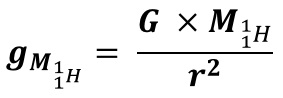
and Compressed Space-Time
Uncompressed
Space-Time
Distance from
Center of Proton
MetersProton
Gravitational
Field
Meters/Second2Proton
Gravitational
Field
Units of
Earth Gravity
gProton
Gravitational Field
Uncompressed
Space-Time
Speed of Light
Meters/SecondSpace-Time
Compression
FactorCompressed
Space-Time
Distance from
Center of Proton
MetersQuantized
Gravitational
Field in
Compressed
Space-Time
Meters/Second2
1.200E-15
2.395E+28
2.441E+27
2.395E+28
7.989E+19
1.200E-15
2.395E+28
2.000E-15
8.621E+27
8.788E+26
8.621E+27
2.876E+19
1.200E-15
8.621E+27
5.000E-15
1.379E+27
1.406E+26
1.379E+27
4.602E+18
1.200E-15
1.379E+27
1.000E-14
3.448E+26
3.515E+25
3.448E+26
1.150E+18
1.200E-15
3.448E+26
2.000E-14
8.621E+25
8.788E+24
8.621E+25
2.876E+17
1.200E-15
8.621E+25
5.000E-14
1.379E+25
1.406E+24
1.379E+25
4.602E+16
1.200E-15
1.379E+25
1.000E-13
3.448E+24
3.515E+23
3.448E+24
1.150E+16
1.200E-15
3.448E+24
2.000E-13
8.621E+23
8.788E+22
8.621E+23
2.876E+15
1.200E-15
8.621E+23
5.000E-13
1.379E+23
1.406E+22
1.379E+25
4.602E+14
1.200E-15
1.379E+23
1.000E-12
3.448E+22
3.515E+21
3.448E+22
1.150E+14
1.200E-15
3.448E+22
2.000E-12
8.621E+21
8.788E+20
8.621E+21
2.876E+13
1.200E-15
8.621E+21
5.000E-12
1.379E+21
1.406E+20
1.379E+21
4.602E+12
1.200E-15
1.379E+21
1.000E-11
3.448E+20
3.515E+19
3.448E+20
1.150E+12
1.200E-15
3.448E+20
2.000E-11
8.621E+19
8.788E+18
8.621E+19
2.876E+11
1.200E-15
8.621E+19
5.000E-11
1.379E+19
1.406E+18
1.379E+19
4.602E+10
1.200E-15
1.379E+19
1.000E-10
3.448E+18
3.515E+17
3.448E+18
1.150E+10
1.200E-15
3.448E+18
2.000E-10
8.621E+17
8.788E+16
8.621E+17
2.876E+09
1.200E-15
8.621E+17
5.000E-10
1.379E+17
1.406E+16
1.379E+17
4.602E+08
1.200E-15
1.379E+17
1.000E-09
3.448E+16
3.515E+15
3.448E+16
1.150E+08
1.200E-15
3.448E+16
2.000E-09
8.621E+15
8.788E+14
8.621E+15
2.876E+07
1.200E-15
8.621E+15
5.000E-09
1.379E+15
1.406E+14
1.379E+15
4.602E+06
1.200E-15
1.379E+15
1.000E-08
3.448E+14
3.515E+13
3.448E+14
1.150E+06
1.200E-15
3.448E+14
2.000E-08
8.621E+13
8.788E+12
8.621E+13
2.876E+05
1.200E-15
8.621E+13
5.000E-08
1.379E+13
1.406E+12
1.379E+13
4.602E+04
1.200E-15
1.379E+13
1.000E-07
3.448E+12
3.515E+11
3.449E+12
1.150E+04
1.200E-15
3.448E+12
2.000E-07
8.621E+11
8.788E+10
8.624E+11
2.877E+03
1.201E-15
8.621E+11
5.000E-07
1.379E+11
1.406E+10
1.382E+11
4.612E+02
1.203E-15
1.379E+11
1.000E-06
3.448E+10
3.515E+09
3.478E+10
1.160E+02
1.214E-15
3.448E+10
2.000E-06
8.621E+09
8.788E+08
8.920E+09
2.976E+01
1.254E-15
8.621E+09
5.000E-06
1.379E+09
1.406E+08
1.679E+09
5.602E+00
1.478E-15
1.379E+09
1.000E-05
3.448E+08
3.515E+07
6.446E+08
2.150E+00
2.166E-15
3.448E+08
1.073E-05
2.998E+08
3.056E+07
5.995E+08
2.000E+00
3.248E-15
2.998E+08
2.000E-05
8.621E+07
8.788E+06
3.860E+08
1.288E+00
3.848E-15
8.621E+07
5.000E-05
1.379E+07
1.406E+06
3.135E+08
1.046E+00
7.526E-15
1.379E+07
1.000E-04
3.448E+06
3.515E+05
3.032E+08
1.012E+00
1.497E-14
3.448E+06
2.000E-04
8.621E+05
8.788E+04
3.006E+08
1.003E+00
1.497E-14
8.621E+05
5.000E-04
1.379E+05
1.406E+04
2.999E+08
1.000E+00
5.977E-14
1.379E+05
1.000E-03
3.448E+04
3.515E+03
2.998E+08
1.000E+00
1.195E-13
3.448E+04
2.000E-03
8.621E+03
8.788E+02
2.998E+08
1.000E+00
2.390E-13
8.621E+03
5.000E-03
1.379E+03
1.406E+02
2.998E+08
1.000E+00
4.781E-13
1.379E+03
1.000E-02
3.448E+02
3.515E+01
2.998E+08
1.000E+00
9.562E-13
3.448E+02
2.000E-02
8.621E+01
8.788E+00
2.998E+08
1.000E+00
1.912E-12
8.621E+01
5.000E-02
1.379E+01
1.406E+00
2.998E+08
1.000E+00
3.825E-12
1.379E+01
5.929E-02
9.810E+00
1.000E+00
2.998E+08
1.000E+00
7.649E-12
9.810E+00
1.000E-01
3.448E+00
3.515E-01
2.998E+08
1.000E+00
1.530E-11
3.448E+00
2.000E-01
8.621E-01
8.788E-02
2.998E+08
1.000E+00
3.060E-11
8.621E-01
5.000E-01
1.379E-01
1.406E-02
2.998E+08
1.000E+00
6.120E-11
1.379E-01
1.000E+00
3.448E-02
3.515E-03
2.998E+08
1.000E+00
1.224E-10
3.448E+00
2.000E+00
8.621E-03
8.788E-04
2.998E+08
1.000E+00
2.448E-10
8.621E-03
5.000E+00
1.379E-03
1.406E-04
2.998E+08
1.000E+00
4.896E-11
1.379E-03
Nuclear Electric Field Outside Nucleus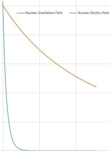
Quantized Light and Photo-Electric Effect Analogous to Quantized Gravity – Liberating Outer Electron from Sodium Atom:
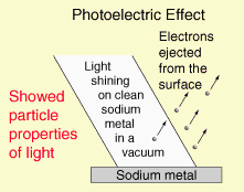
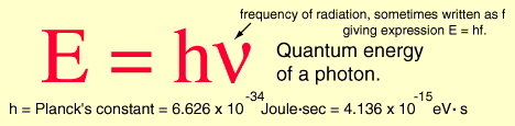
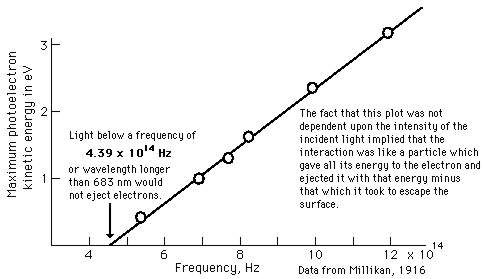
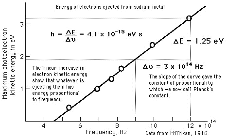
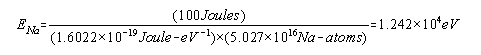
![]()
![]()
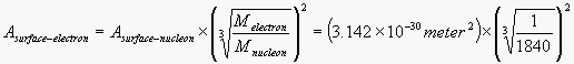
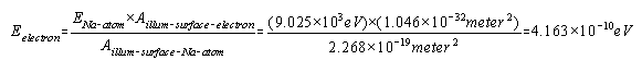
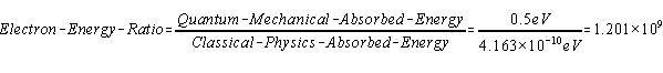
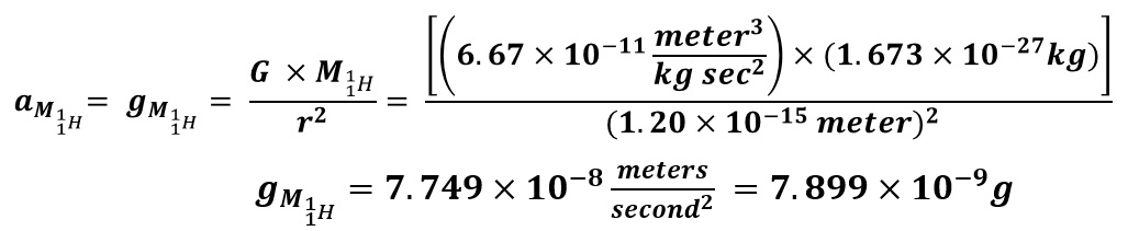
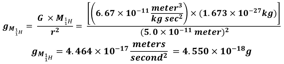
Strong Nuclear Force Properties Provide Case for Equivalence to Gravity
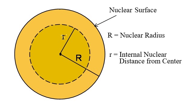
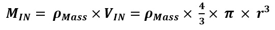
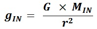
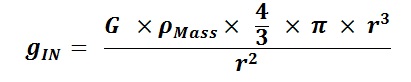
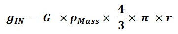
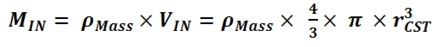
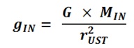
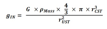
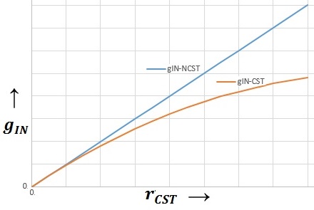
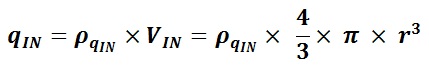
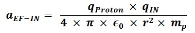
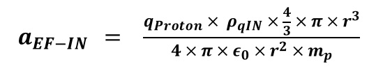
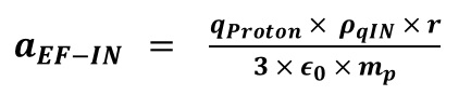
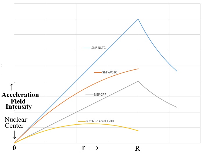
SNF-WSTC = Strong Nuclear Force - (If Gravity) With Space-Time Compression
NEF-CRP = Nuclear Electric Field - Coulombic Repulsion Protons
Net Nuc Accel Field = Net Nuclear Acceleration Field = [SNF-WSTC] - [NEF-CRP]
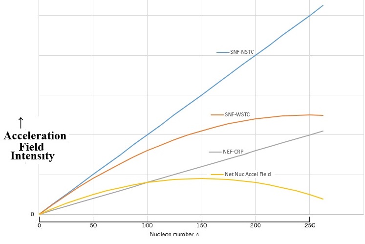
SNF-WSTC = Strong Nuclear Force - (If Gravity) With Space-Time Compression
NEF-CRP = Nuclear Electric Field - Coulombic Repulsion Protons
Net Nuc Accel Field = Net Nuclear Acceleration Field = [SNF-WSTC] - [NEF-CRP]
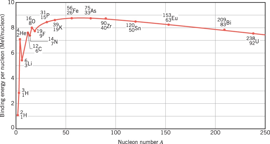
Nuclear Gravitation Field and Configuration of Lead-208 and Bismuth-209
for Lead (Pb-208) and Bismuth (Bi-209)
Energy
Level1
(He)2
(O)3
(Ca)4
(Ni)5
(Sn)6
(Pb)7
(Fl)8
(E164)Total
Protons
and
Neutrons
Protons
Lead
(82Pb208)
Neutrons2p
2n6p
6n12p
12n8p
8n22p
22n32p
32n
44n
82p
126n
Protons
Bismuth
(83Bi209)
Neutrons2p
2n6p
6n12p
12n8p
8n22p
22n32p
32n1p
44n
83p
126n
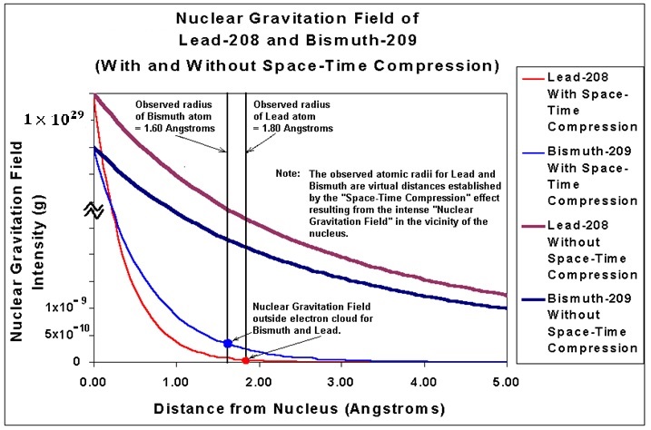
6.6726 x 10⁻¹¹ Newton-meter2/kg2 (= 6.6726 x 10⁻¹¹ meter3/kg-sec2). If the outcome of performing these Cavendish Experiments results in determining that the value for GBi is greater than the value for G (Universal Gravitation Constant) which is greater than the value for GPb, then this outcome will provide compelling evidence the Strong Nuclear Force and Gravity are one and the same. The Universal Gravitation Constant is, therefore, not Universal but specific to every isotope of every Element. It is related to the Binding Energy Per Nucleon and does not vary much for stable isotopes of Elements. The exceptions are Lead-208, a tight fitting “double magic” nucleus containing a strong Nuclear Gravitation Field next to its nucleus and Bismuth-209, containing a “loosely held” single proton in an outer energy level with a magic number for neutrons containing a relatively weak Nuclear Gravitation Field next to its nucleus.
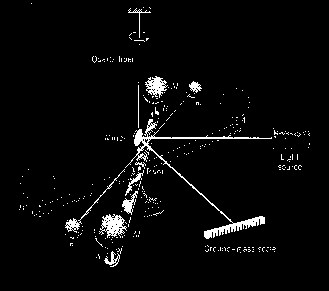
The Cavendish balance, used for experimental verification of Newton's Law of Universal Gravitation. Masses m and m are suspended from a quartz fiber. Masses M and M can rotate on a stationary support. An image of the l amp filaments is reflected by the mirror attached to m and m onto the scale so that any rotation of m and m can be measured.
Reference: “Physics, Parts I and II,” David Halliday and Robert Resnick
Originating from Nucleus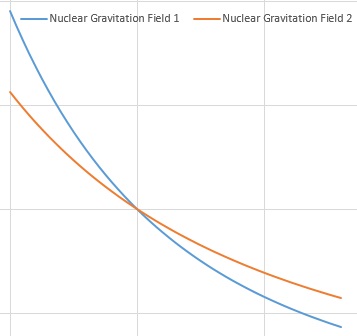
Conclusion
![]()
![]()
NUCLEAR GRAVITATION FIELD THEORY AUTHOR
KENNETH F. WRIGHT (KEN) BACKGROUND
![]()
EDUCATION
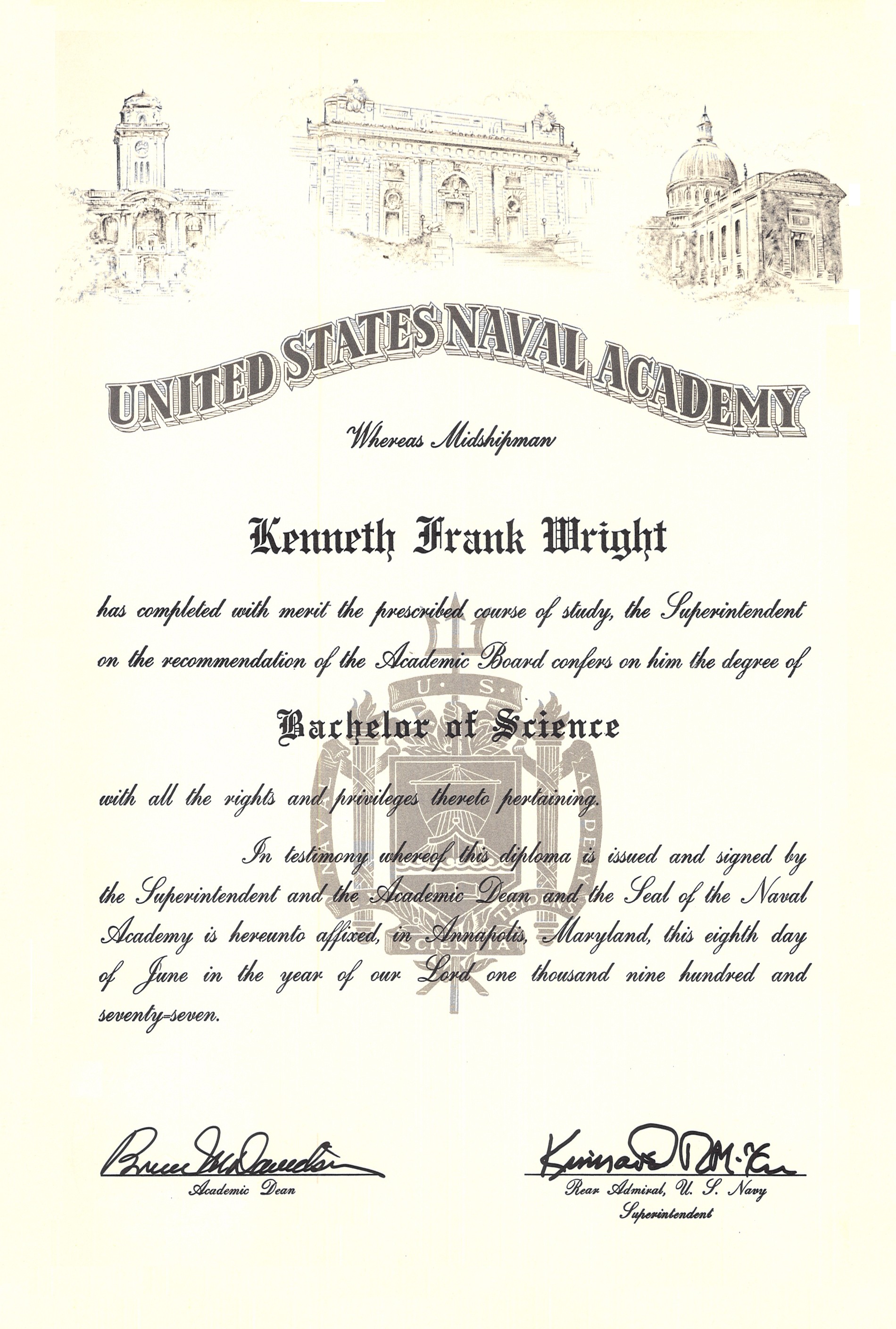
USNA Bachelor of Science Degree
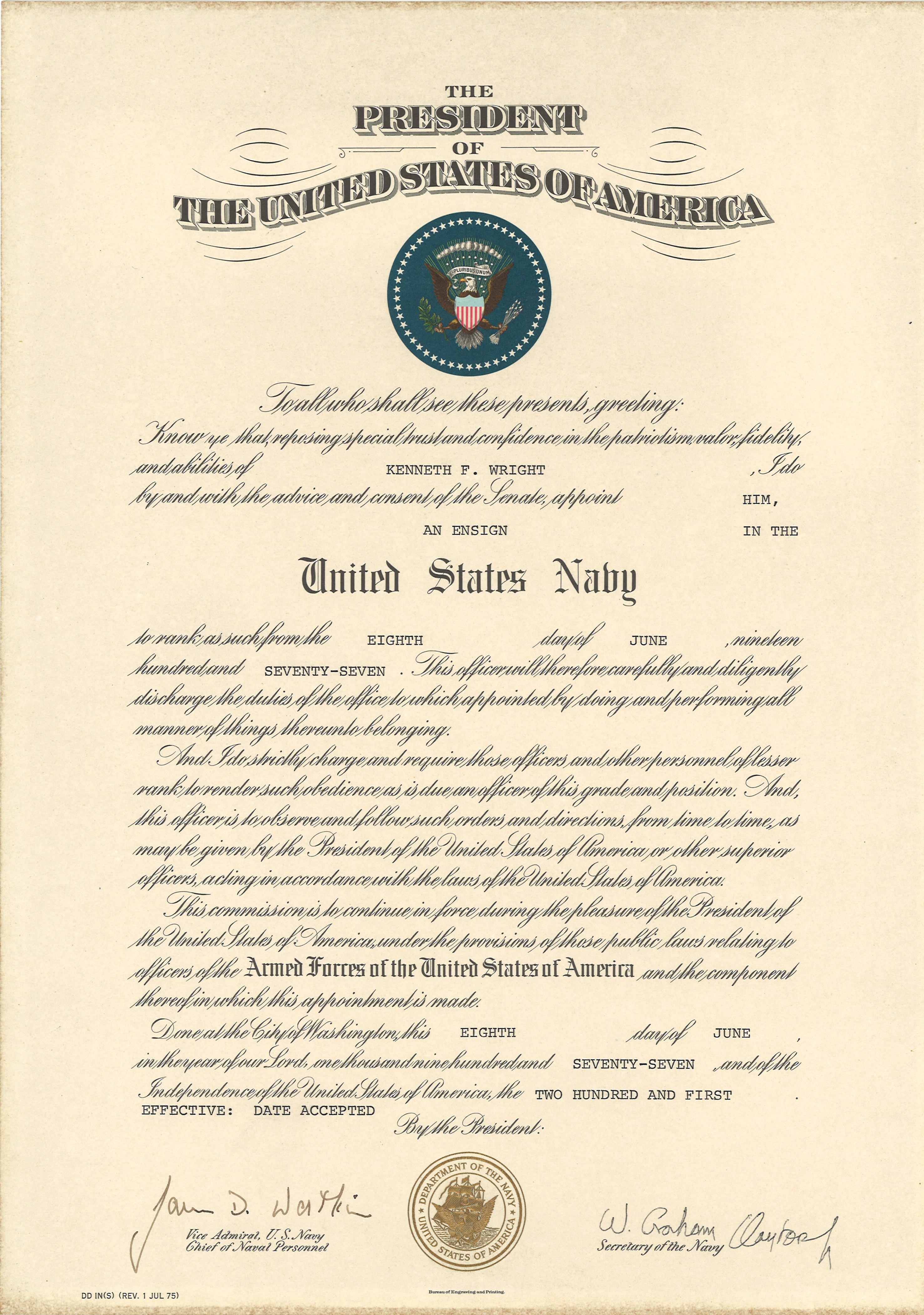
Commissioning as US Naval Officer
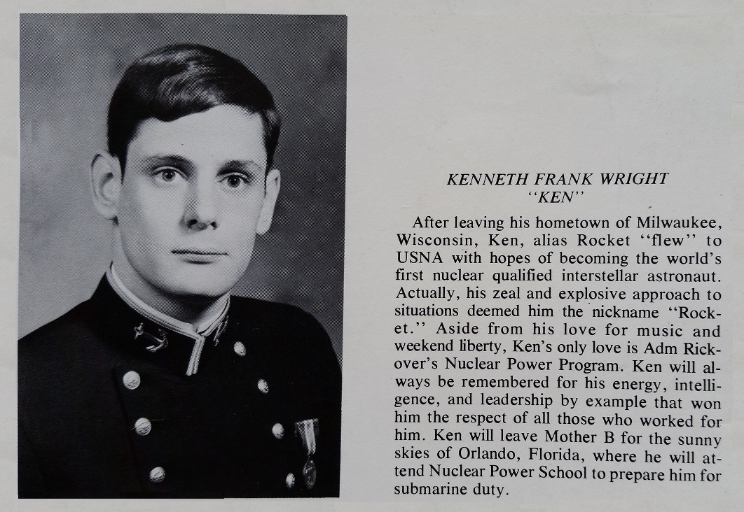
Midshipman Kenneth Frank Wright
U. S. Naval Academy Class of 1977 Yearbook Entry
![]()
United States Naval Academy Logo
USNA Class of 1977 Class Crest


United States Naval Academy
Annapolis, Maryland

Naval Reactors Facility
Idaho National Engineering Laboratory

Groton, Connecticut


University of Phoenix - San Diego, California
![]()
WORK HISTORY


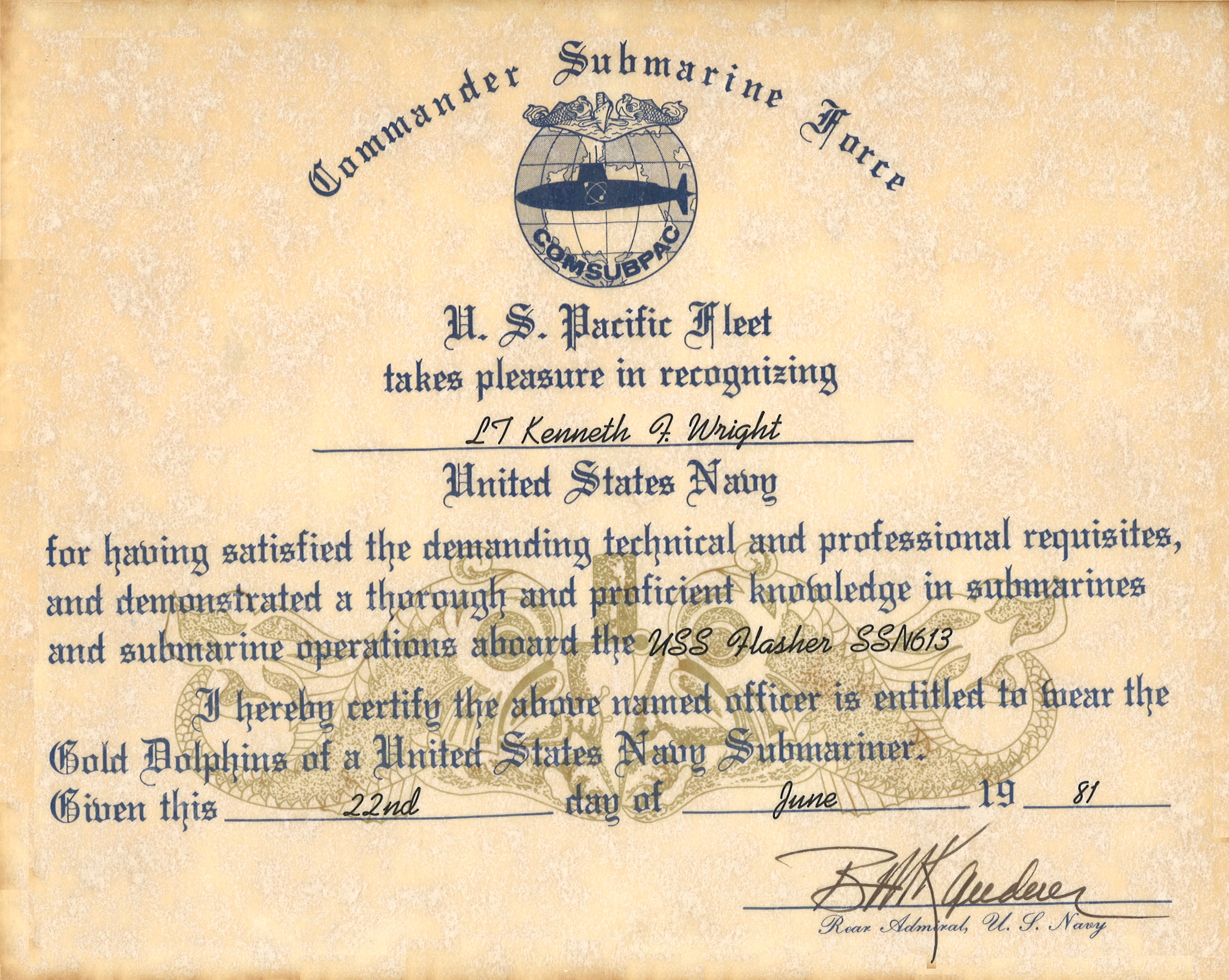

U.S. Naval Officer’s Gold Dolphins
Qualified in Submarines
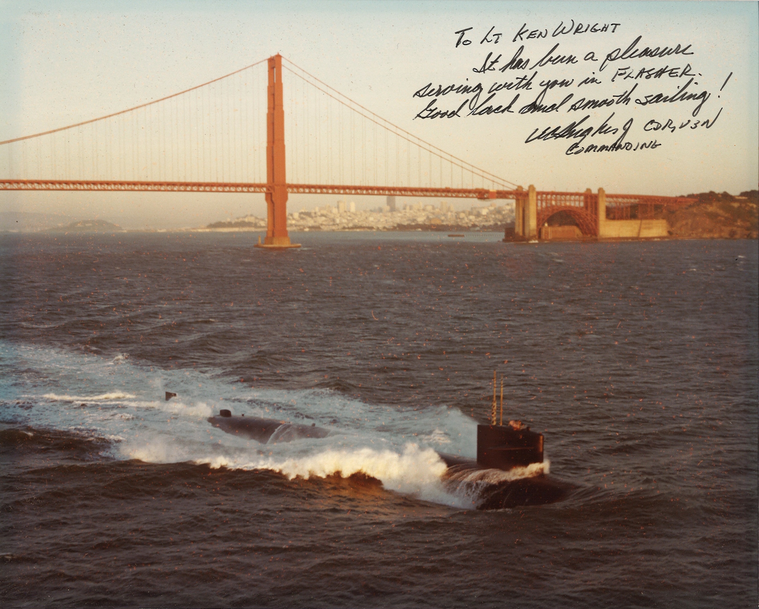
U.S.S. Flasher (SSN-613)
Nuclear Powered Fast Attack Submarine
Best in the West
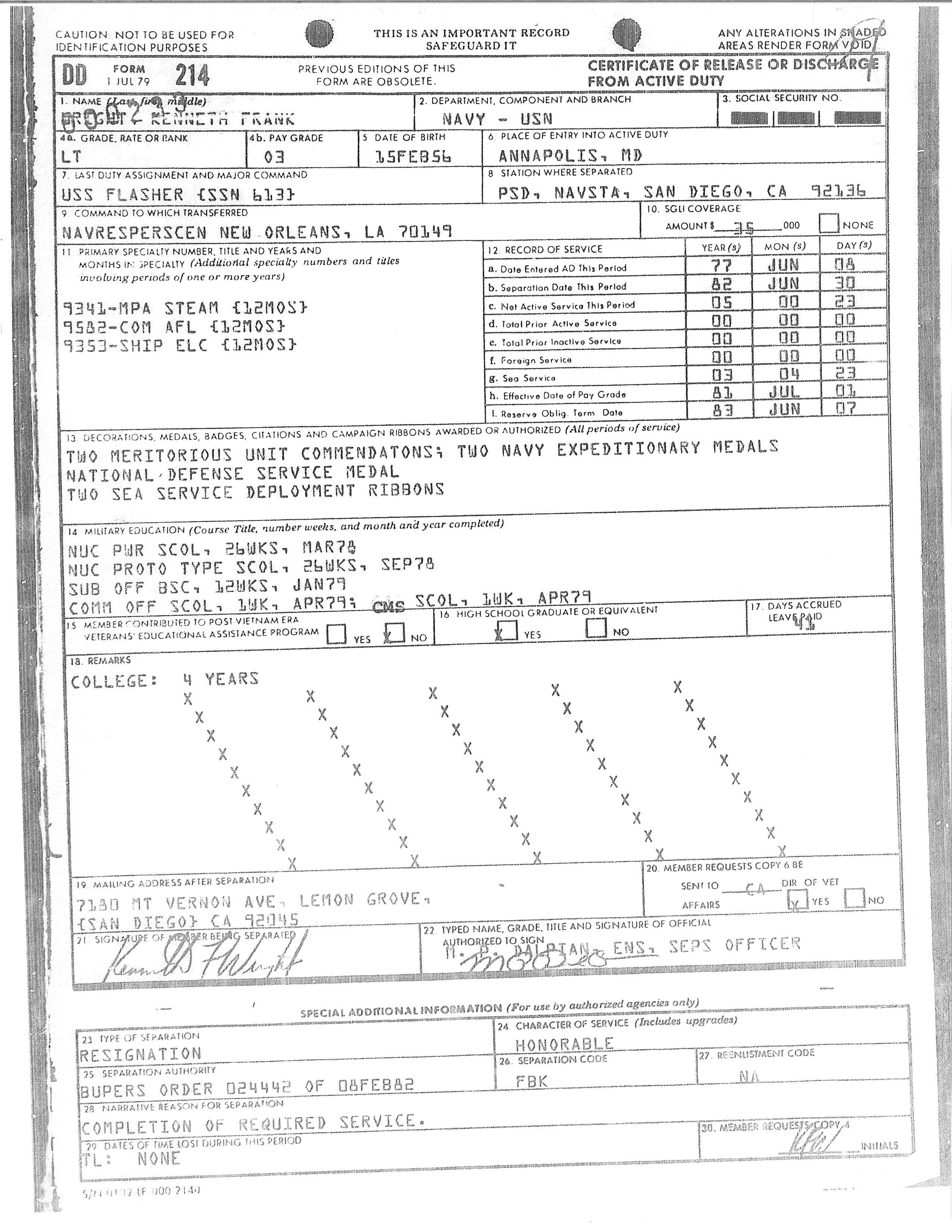
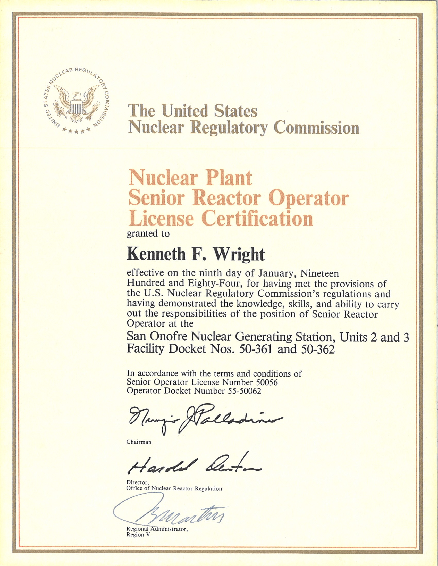
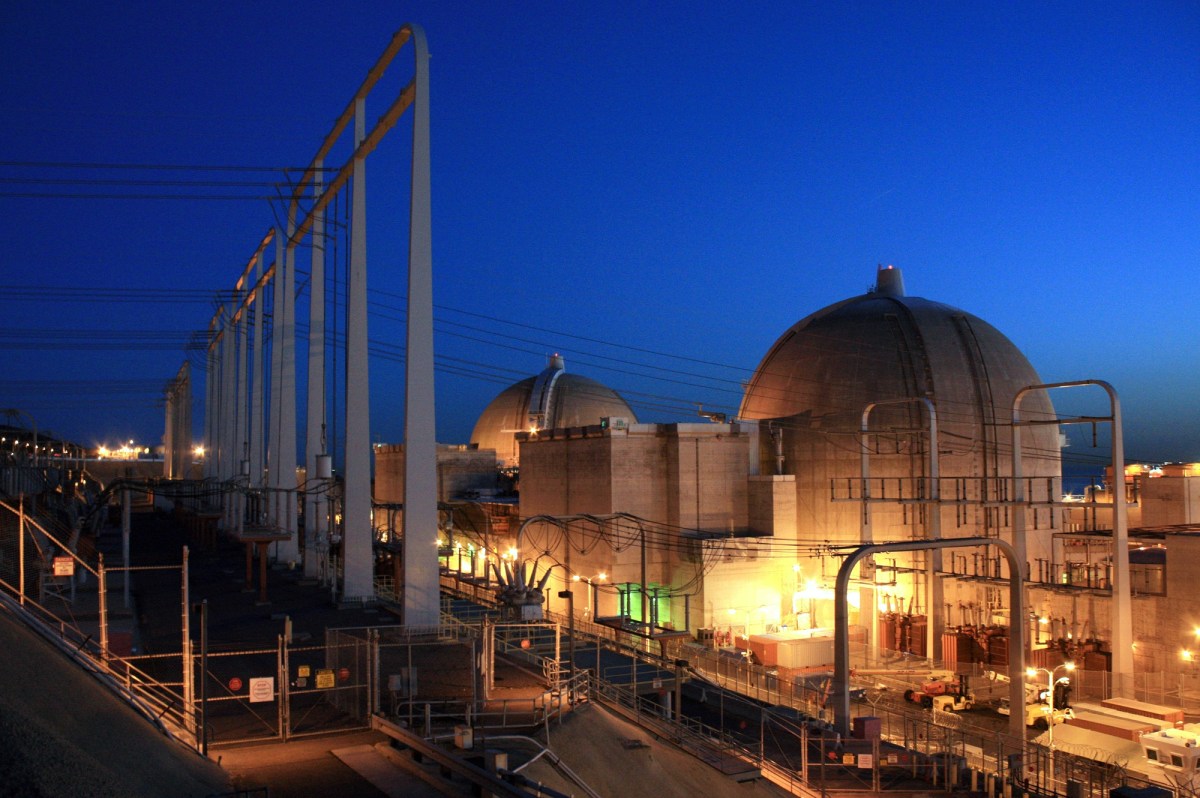
San Onofre Nuclear Generating Station
Units 2 and 3
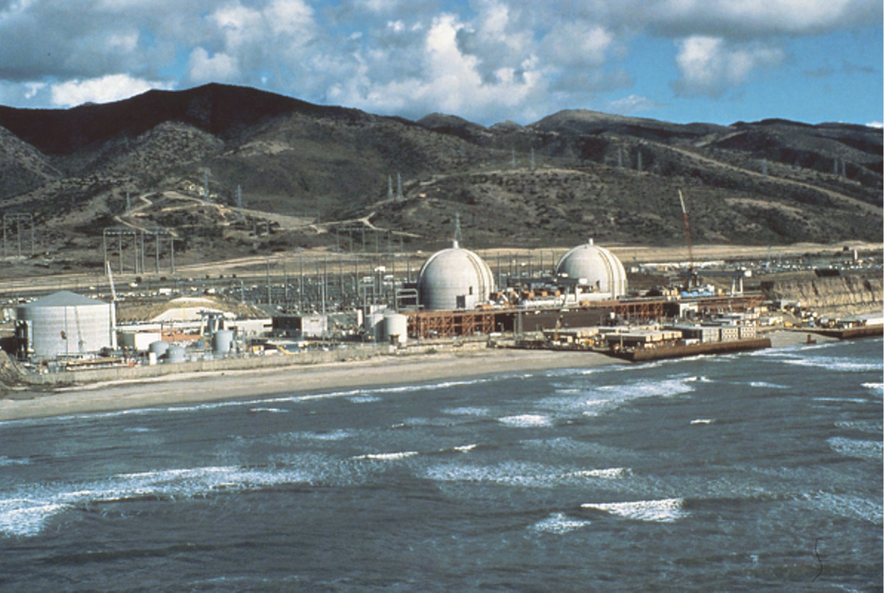
San Onofre Nuclear Generating Station - San Clemente, California

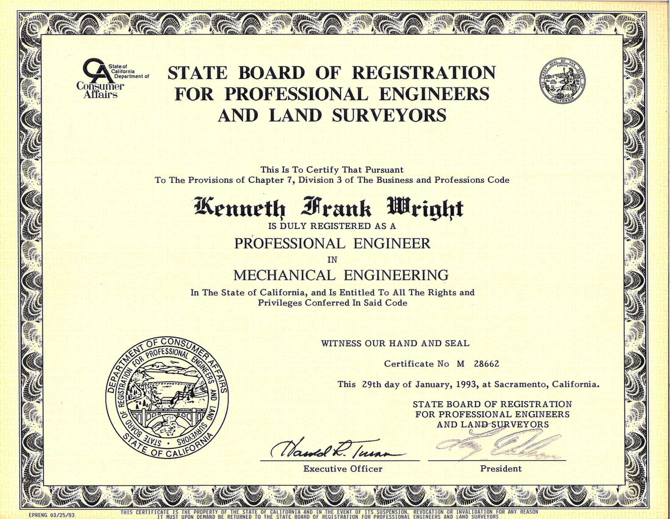
![]()
South Texas Project Nuclear Electric Generating Station
Wadsworth, Texas

Duke Energy Corporate Offices
Charlotte, North Carolina
Duke Energy Building at Night
Celebrating Independence Day
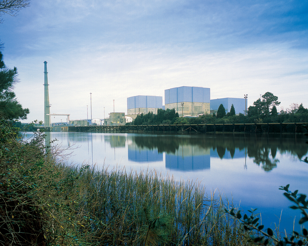
Brunswick Nuclear Plant
Southport, North Carolina
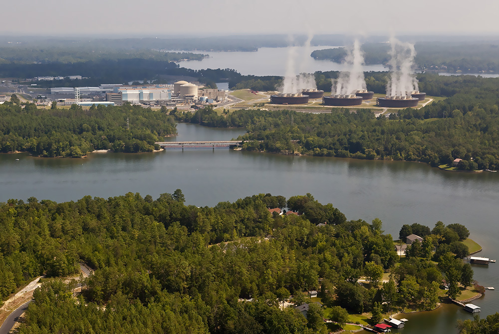
Catawba Nuclear Station
York, South Carolina
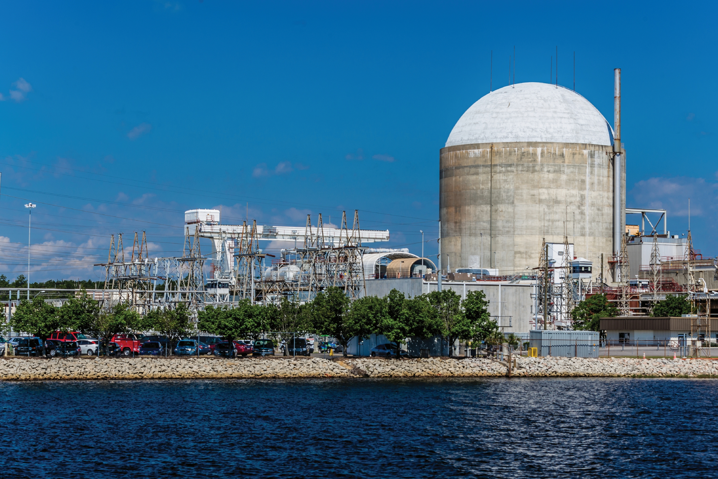
H. B. Robinson Nuclear Plant
Hartsville, South Carolina

McGuire Nuclear Station
Huntersville, North Carolina
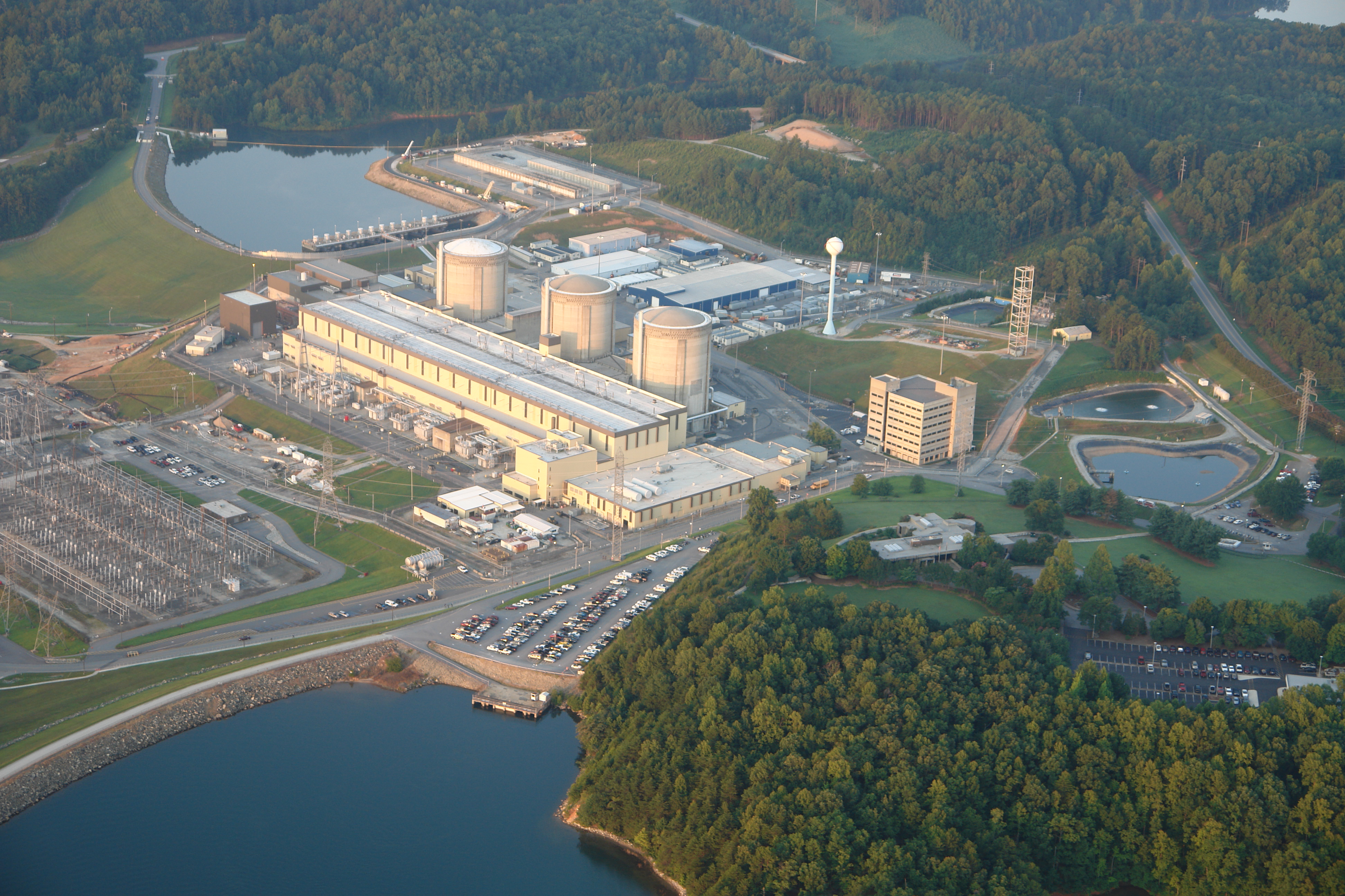
Oconee Nuclear Station
Seneca, South Carolina
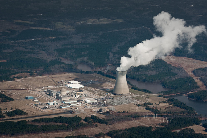
Shearon-Harris Nuclear Plant
New Hill, North Carolina
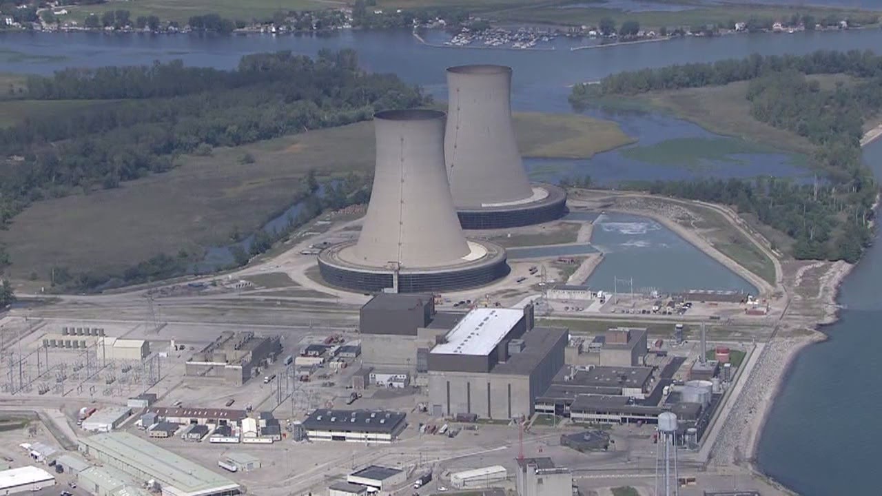
Enrico Fermi Nuclear Plant
Newport, Michigan

Jackson SRS Security Entrance Gate

Savannah River Site - H Area
.United States Department of Energy - Savannah River Site
Aiken, South Carolina

Duke Energy Generation Support Facility
Kings Mountain. North Carolina
![]()

Kenneth F. Wright (Ken) Background
Adobe Acrobat pdf Format
Background Full Page Images
Adobe Acrobat pdf Format
![]()
![]()
![]()
![]()
All rights reserved. No portion of this document may be reproduced
in any form without written permission of the author.